A 1-D time-varying median filter for seismic random, spike-like noise elimination

Processing of field data

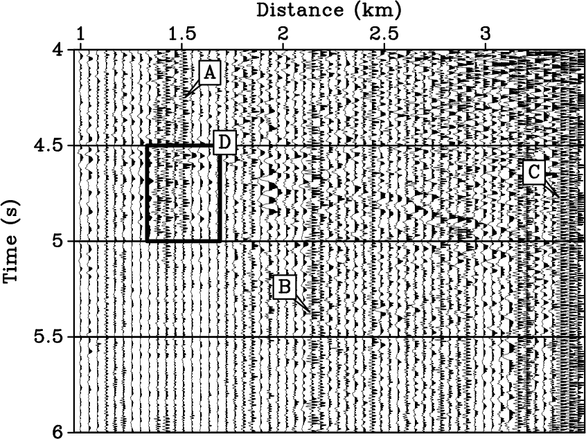
A real-data example involves land prestack data from Texas (Figure 6a), from which we show one common midpoint gather that has 59 traces and an average group interval of 42 m. The sample frequency is 4 ms, and the sample number is 500. In Figure 6a, noise is mainly random noise caused by the surface condition of this area; the 60-Hz electrical interference with high amplitude is especially serious. According to the amplitude spectra, the dominant frequency of the real data is about 25 Hz; the 60-Hz electrical interference thus exhibits high-frequency, spike-like characteristics when compared with the useful signal. In the time domain (Figure 6a, especially at locations ``A,'' ``B,'' and ``C''), this spike-like characteristic of electrical interference can also be observed. 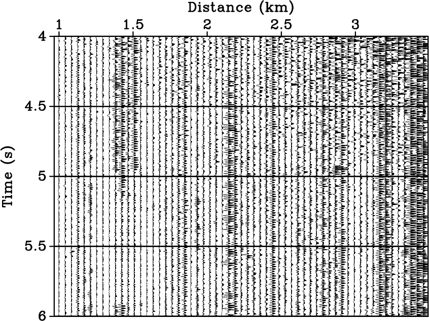To meet the assumptions of SNR estimation using the stack method, a rectangle region ``D'' that has 9 traces and 125 samples is chosen, and, after calculating, the SNR in the original data is found to be -7.3 dB. First, we apply a low-pass filter to remove the random noise (Figure 6b); the frequency is limited to 60 Hz. The low-pass filter can partly eliminate random noise, and the corresponding SNR is improved to 0.4 dB, but it cannot attenuate the noise in the dominant-frequency band. We can thus still see lots of random noise after filtering. The 11-point stationary MF is also used to compare with the TVMF, and the result is shown in Figure 6c. After processing, there is still some spike-like noise left, and part of the signal has been attenuated. The SNR is 1.9 dB, and a larger filter window will further destroy the useful signal. By using the SNR analysis introduced in the theory section, we are choosing the parameters about the TVMF in window ``D.'' The TVMF with the same parameters as for the synthetic examples, $C=11$, $\alpha=2$, $\beta=0$, $\gamma=4$, and $\delta=6$, is applied to the prestack data (Figure 6d). Figure 6e shows the difference section, in which the processed data using the TVMF have been subtracted from the original data. After TVMF processing, continuity of events and information of the reflected waves are all enhanced, and there is little noise left. Note that the 60-Hz electrical interference in particular can be completely removed. The SNR reaches 4.7 dB. In the difference section it can be seen that the TVMF eliminates major spike-like noise and that there is little useful information beyond the spike-like noise, showing that the TVMF can effectively eliminate spike-like noise and protect useful information at the same time. Because the TVMF is based on the stationary MF that can filter noise spikes, the TVMF can effectively eliminate spike-like noise. And because the TVMF can separate useful information from spike-like noise, it can protect useful information and perform better overall than other potential methods in spike-like noise attenuation.

dragon1,band,11mf,11tvmf,diff
Figure 6. Real land data (a), denoised result after low-pass filtering (b), denoised result after stationary MF filter (c), denoised result after TVMF filtering (d), and difference between original data and result after TVMF processing (e).

We chose a trace from the original data and corresponding traces in processed data and got the amplitude spectra of four traces (Figure 7). After low-pass filtering, high-frequency noise can be removed thoroughly, but some noise in the dominant-frequency band can remain; electrical interference in particular must be eliminated by other methods (Figure 7b). Stationary MF can eliminate enough noise, but spectra of useful signals have been distorted (Figure 7c). In Figure 7d, the TVMF can attenuate noise in the entire frequency band and protect the useful-information frequency components.

dspec,bspec,mfspec,fspec
Figure 7. Comparison of amplitude spectra (trace at distance of 1.8 km) before and after processing. Amplitude spectra in Figure 6a (a), corresponding spectra in Figure 6b (b), corresponding spectra in Figure 6c (c), and corresponding spectra in Figure 6d (d).

Next we obtained stacked sections corresponding to Figure 6b and 6d; the stacking fold is 59. A rectangular region, ``H,'' was chosen to calculate the local SNR. Events of the stacked section using low-pass processing were discontinuous (Figure 8a), the SNR is -7.8 dB, and the continuity of events in the stacked section using TVMF processing was improved, especially at locations ``E,'' ``F,'' and ``G'' (Figure 8b), and the corresponding SNR is -3.1 dB. Because the TVMF can eliminate spike-like noise in prestack data, it is advantageous to apply to such data.

stack1,stack2
Figure 8. Stacked section of prestack data after low-pass filtering (a) and corresponding section after TVMF processing (b).

A 1-D time-varying median filter for seismic random, spike-like noise elimination