Kirchhoff migration using eikonal-based computation of traveltime source-derivatives

Traveltime Source-derivative

The point-source traveltime $T(\mathbf{x})$ clearly depends on the source location $\mathbf{x_s}$. To explicitly show such a dependency in the eikonal equation, we define a relative coordinate $\mathbf{q}$ as

$$\mathbf{q = x - x_s}\;,$$ (2)

and use $\hat{T}(\mathbf{q};\mathbf{x_s})$ to denote traveltime in the relative coordinates. After inserting this definition into equation 1, we obtain

$$\nabla_{\mathbf{q}} \hat{T} \cdot \nabla_{\mathbf{q}} \hat{T} = W (\mathbf{q+x_s})\;.$$ (3)

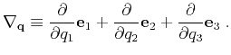
Here the differentiation $\nabla_{\mathbf{q}}$ stands for gradient operator in the relative coordinate $\mathbf{q}$ and is taken with a fixed source location $\mathbf{x_s}$. In 3D, if $\mathbf{q} = (q_1,q_2,q_3)$ and denoting $\mathbf{e}_i$ with $i = \{1,2,3\}$ to be the unit vector in depth, inline and crossline directions, respectively, then

$$\nabla_{\mathbf{q}} \equiv \frac{\partial}{\partial q_1} \mathbf... ...ial}{\partial q_2} \mathbf{e}_2 + \frac{\partial}{\partial q_3} \mathbf{e}_3\;.$$ (4)

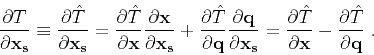
Since we are interested in the traveltime derivative with respect to the source, i.e. $\partial T / \partial \mathbf{x_s}$, we take directional derivative $\partial / \partial \mathbf{x_s}$ to $\hat{T}(\mathbf{q};\mathbf{x_s})$ and apply the chain-rule according to equation 2:

$$\frac{\partial T}{\partial \mathbf{x_s}} \equiv \frac{\parti... ... \mathbf{x}} - \frac{\partial \hat{T}}{\partial \mathbf{q}}\;.$$ (5)

Equation 5 results in a vector that contains the traveltime source-derivatives in depth, inline and crossline directions. In accordance with $\partial / \partial \mathbf{x_s}$, $\partial / \partial \mathbf{x}$ and $\partial / \partial \mathbf{q}$ are also directional derivatives. All numerical examples in this paper are based on a typical 2D acquisition, where we assume a constant source depth and thus only the inline traveltime source-derivative is of interest. The quantity $\partial \hat{T} / \partial \mathbf{q}$ coincides with the slowness vector of the ray that originates from $\mathbf{x_s}$. For a finite-difference eikonal solver such as FMM and FSM, it is usually estimated by an upwind scheme during traveltime computations at each grid point and thus can be easily extracted. Applying $\partial / \partial \mathbf{x}$ to both sides of equation 3, we find

$$\nabla_{\mathbf{q}} \hat{T} \cdot \nabla_{\mathbf{q}} \frac... ...f{x}} = \frac{1}{2} \frac{\partial W}{\partial \mathbf{x}}\;.$$ (6)

Equation 6 has the form of the linearized eikonal equation (Aldridge, 1994) and was previously derived, in a slightly different notation, by Alkhalifah and Fomel (2010). It implies that $\partial \hat{T} / \partial \mathbf{x}$, as needed by equation 5, can be determined along the characteristics of $\hat{T}$. Since the right-hand side contains a slowness-squared derivative, the velocity model must be differentiable, as is usually required by traveltime computations. The derivation also indicates that the accuracy of an eikonal-based traveltime source-derivative is source-sampling independent but model-sampling dependent, as from equations 5 and 6 $\partial / \partial \mathbf{x_s}$ relies on $\hat{T}$, $\partial / \partial \mathbf{q}$ and $\partial / \partial \mathbf{x}$. The accuracy from a direct finite-difference estimation on $\partial / \partial \mathbf{x_s}$, in comparison, is both source- and model-sampling dependent.

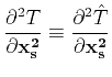
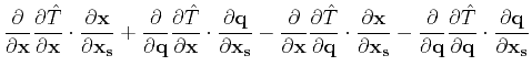
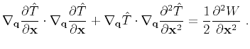
Continuing applying differentiation and the chain-rule to equation 5 will result in higher-order traveltime source-derivatives. For example, the second-order derivative reads:

$$\frac{\partial^2 T}{\partial \mathbf{x_s^2}} \equiv \frac{\partial^2 \hat{T}}{\partial \mathbf{x_s^2}} = \frac{\partial}{\partial \mathbf{x}} \frac{\partial \hat{T}}{\par... ...}{\partial \mathbf{q}} \cdot \frac{\partial \mathbf{q}}{\partial \mathbf{x_s}}$$

$$= \frac{\partial^2 \hat{T}}{\partial \mathbf{x}^2} - 2 \frac{\part... ...{x} \partial \mathbf{q}} + \frac{\partial^2 \hat{T}}{\partial \mathbf{q}^2}\;.$$ (7)

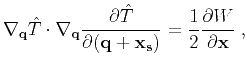
Further, differentiating equation 6 once more by $\mathbf{x}$ provides

$$\nabla_{\mathbf{q}} \frac{\partial \hat{T}}{\partial \mathbf{x}} ... ...tial \mathbf{x}^2} = \frac{1}{2} \frac{\partial^2 W}{\partial \mathbf{x}^2}\;.$$ (8)

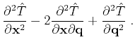
It is easy to verify that any order of the traveltime source-derivative will require the corresponding order of the slowness-squared derivative. An approximation based on Taylor expansions of the traveltime around a fixed source location can make use of these derivatives. For example, Ursin (1982) and Bortfeld (1989) introduced parabolic and hyperbolic traveltime approximations with the first- and second-order derivatives. Notice that the need for slowness-squared derivatives may cause instability unless the velocity model is sufficiently smooth. Alkhalifah and Fomel (2010) also proved the following relationship between $\partial W/\partial \mathbf{x}$ and $\partial \hat{T} / \partial \mathbf{q}$:

$$\nabla_{\mathbf{q}} \hat{T} \cdot \nabla_{\mathbf{q}} \frac{\par... ...tial \mathbf{(q+x_s)}} = \frac{1}{2} \frac{\partial W}{\partial \mathbf{x}}\;,$$ (9)

which implies that the traveltime source-derivative can be computed from the given traveltime tables only. However, the velocity smoothness is still implicitly assumed as the second-order spatial derivatives of traveltimes appear in the equation. For this reason, we restrict our current implementation to the first-order derivative only.

In a ray-tracing eikonal solver, $\partial T / \partial \mathbf{x_s}$ is the slowness vector of a particular ray at $\mathbf{x_s}$ and holds constant along the trajectory. As it may also require irregular coordinate mappings, one may use the same strategy as for the traveltime tables. In this way, there is no necessity for any additional effort. On the other hand, equations 5 and 6 and their second-order extensions provide important attributes for use in Gaussian beams, which are commonly calculated by the dynamic ray tracing (Cervený, 2001). They might be alternatively estimated by the eikonal-based source-derivative formulas but with the traveltime tables from a finite-difference eikonal solver. However, this application is beyond the scope of this paper. In the following sections, we consider only the source-derivative estimation from traveltimes computed by a finite-difference eikonal solver.

Kirchhoff migration using eikonal-based computation of traveltime source-derivatives