Examples

The first synthetic example is shown in Figures 3, 4, 5, 6 and 7. Figure 3a shows the original well-sampled data. By regularly removing 50 % traces, we simulate the under-sampled data and show it in Figure 3b. After using the proposed approach, we obtain a perfect reconstructed data as shown in Figure 4a. The dip estimation is applied on the low-frequency data using 15 Hz low-pass filtering. During each iteration, we preserve 8% coefficients. In order to numerically compare the denoising performances of different approaches, we utilize the signal-to-noise ratio (SNR) Chen et al. (2015):

$$SNR_n=10\log_{10}\frac{\Arrowvert \mathbf{m} \Arrowvert_2^2}{\Arrowvert \mathbf{m}-\mathbf{m}_n\Arrowvert_2^2},$$ (9)

where $\mathbf{m}$ is the original complete data and $\mathbf{m}_n$ is denotes the reconstructed data after $n$th iteration. After 200 iterations, we obtain a well-reconstructed data with a high SNR: 28.02 dB. Figure 7 shows the convergence diagram in terms of SNR using the proposed approach. It is clear that the percentile thresholding strategy can help obtain a converged result with a high SNR. Figures 3c and 3d show the $F-K$ spectrum of the original data and decimated data. It is obvious that the removed traces cause strong spatial aliasing in the spectrum (Figure 3d). We also use the traditional $F-X$ prediction based approach Spitz (1991) to interpolate the decimated data and show the result in Figure 4b. The performance of $F-X$ prediction method also obtains a good recovery of the missing traces. However, when compared in the $F-K$ domain (Figures 4c and 4d), the proposed approach clearly does a better job because there is still some aliasing noise left in the spectrum from $F-X$ prediction method. It can be further confirmed from the interpolation error sections, as shown in Figure 5. $F-X$ prediction method causes noticeable estimation error while the proposed approach causes nearly zero error.

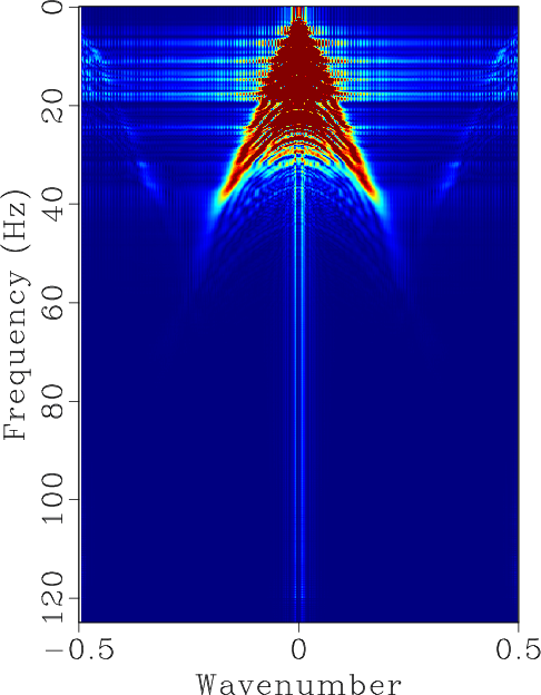
As we can see, the spectrum of the reconstructed data using the proposed approach is exactly the same as the original data. If we use a filter with a somewhat higher low-pass frequency, we will obtain a much worse reconstructed result, because of the severe aliasing problem. Figure 6a shows the precise dip estimation from the original data. Figure 6b shows the final dip estimation using 15 Hz low-pass filtering. The final dip estimation using 30 Hz low-pass filtering shows incorrect dips around 0.75 s at trace 250 (Figure 6c).

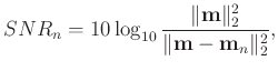
The second synthetic example is a linear-event example to test the performance of the proposed approach on post-stack data. The original data is shown in Figure 8a. We also remove 50% traces regularly. In this example, we compare the proposed approach with the $F-K$ based POCS approach. The reconstructed results using the proposed approach and the $F-K$ based POCS approach are shown in Figures 8c and 8d, respectively. It is obvious that the proposed can still obtain a perfect performance, while the $F-K$ based POCS approach cannot obtain any improvement because of the strong aliasing noise in the $F-K$ domain. This test confirms the fact that $F-K$ based POCS approach should not be used to interpolate regularly missing traces Spitz (1991); Naghizadeh and Sacchi (2007,2010). In this example, we use 100 iterations to obtain the reconstructed results of both seislet and Fourier transforms. The final SNR of the proposed approach reaches 22.47 dB, and the SNR of the $F-K$ based POCS approach stays unchanged: 3.007 dB. The slightly worse performance of the proposed approach on this example than the first example is because the crossing seismic events cause some errors when estimating the local slope, which affect the final performance a bit.

hyper,hyper-zero,fk-hyper,fk-hyper-zero
Figure 3. (a) Original synthetic data. (b) Decimated data (50% traces regularly removed). (c) $F-K$ spectrum of original synthetic data. (d) $F-K$ spectrum of decimated data.

hyper-seis,hyper-fx,fk-hyper-seis,fk-hyper-fx
Figure 4. (a) Reconstructed data using the proposed approach. (b) Reconstructed data using Spitz's approach. (c) $F-K$ spectrum of reconstructed data using the proposed approach. (d) $F-K$ spectrum of reconstructed data using Spitz's approach.

hyper-seis-dif,hyper-fx-dif
Figure 5. (a) Reconstruction error using the proposed approach. (b) Reconstruction error using the Spitz's approach.

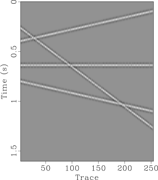
dip,dip1,dip2
Figure 6. (a) Accurate dip estimation. (b) Final dip estimation using 15 Hz low-pass filtering. (c) Final dip estimation using 30 Hz low-pass filtering. Note the aliased dip in (c).

snrs-pocs
Figure 7. Convergence diagram of the first example using the proposed approach.

linear,linear-zero,linear-seis,linear-fft
Figure 8. Second synthetic example test. (a) Original synthetic data. (b) Decimated data (50% traces regularly removed). (c) Reconstructed data using the proposed approach. (d) Reconstructed data using $F-K$ based POCS approach. Note that the $F-K$ based POCS approach cannot obtain any improvement because of the aliasing noise caused by the regularly missing traces.

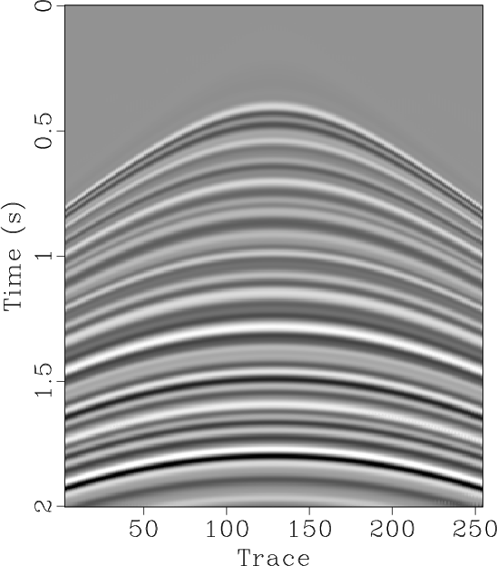
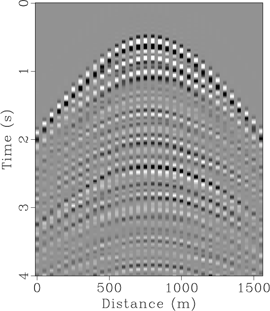
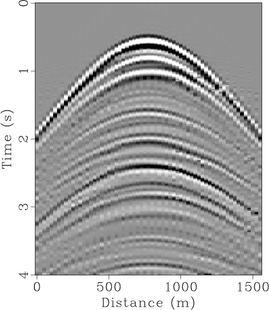
The field data example is a highly under-sampled common shot gather, as shown in Figure 9a. By manually adding zero traces between two neighbor traces, we obtain the zero-padded data, as shown in Figure 9b. After interpolation, a much better sampled data can be obtained, as shown in Figure 9c. In this example, we estimate the local slope using 5 Hz low-pass filtering. The corresponding $F-K$ spectrum are shown in Figures 9d, 9e and 9f, respectively. For many real seismic data, we might have difficulties to get the low-frequency information because of the low SNR at low frequencies. Thus, the proposed approach set a relatively high demand for data quality. Fortunately, we only require the low-frequency data for slope estimation and the appropriate frequency range varies from 5 Hz to 20 Hz for different datasets, which is not a problem for most field dataset.

field,field-zero,field-seis,fk-field,fk-field-zero,fk-field-seis
Figure 9. (a) Original field data. (b) Zero-padded field data. (c) Interpolated field data. (d) $F-K$ spectrum of original field data. (e) $F-K$ spectrum of zero-padded field data. (f) $F-K$ spectrum of interpolated field data.