Solution steering with space-variant filters

Steering Filters

At this point a discussion of steering filters is appropriate. Plane waves with a given slope on a discrete grid can be predicted (destroyed) with compact filters (Schwab, 1997). Inverting such a filter by the helix method, we can create a signal with a given arbitrary slope extremely quickly. If this slope is expected in the model, the described procedure gives us a very efficient method of preconditioning the model estimation problem, fitting goal (2).

How can a plane prediction (steering) filter be created? On the helix surface, the plane wave $P(t,x) = f (t - p x)$ translates naturally into a periodic signal with the period of $T = N_t + \sigma$, where $N_t$ is the number of points on the $t$ trace, and $\sigma = \frac{p \triangle x}{\triangle t}$, where $\sigma$ is the plane slope, and $\triangle x$ and $\triangle t$ correspond to the mesh size. If we design a filter that is two columns long (assuming the columns go in the $t$ direction), then the plane prediction problem is simply connected with the interpolation problem: to destroy a plane wave, shift the signal by $T$, interpolate it, and subtract the result from the original signal. Therefore, we can formally write

$$\mathbf{P} = I - \mathbf{S}(\sigma)\;,$$ (6)

where $\mathbf{P}$ denotes the steering filter, $\mathbf{S}$ is the shift-and-interpolation operator, and $\mathbf{I}$ is the identity operator.

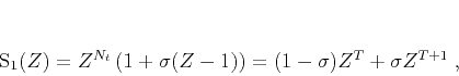
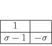
Different choices for the operator $\mathbf{S}$ in (6) produce filters with different length and prediction power. A shifting operation corresponds to the filter with the $Z$-transform $\Sigma(Z) = Z^T$, while the operator $\mathbf{S}$ corresponds to an approximation of $\Sigma(Z)$ with integer powers of $Z$. One possible approach is to expand $\Sigma(Z) Z^{-N_t}$ using the Taylor series around the zero frequency ($Z=1$). For example, the first-order approximation is

$$S_1(Z) = Z^{N_t} \left(1 + \sigma (Z-1)\right) = (1-\sigma) Z^T + \sigma Z^{T+1}\;,$$ (7)

which corresponds to linear interpolation and leads in the two-dimensional space to the steering filter $\mathbf{P}$ of the form

$$\begin{array}{\vert c\vert c\vert} \hline 1 & \hline \sigma-1 & -\sigma \hline \end{array}$$ (8)

Filter (8) is equivalent to the explicit first-order upwind finite-difference scheme on the plane wave equation

$${\frac{\partial P}{\partial x}} + p {\frac{\partial P}{\partial t}} = 0\;.$$ (9)

An important property of filter (8) is that it produces an exact answer for $\sigma=0$ and $\sigma=1$. The values of $\sigma > 1$ lead to unstable inversion. For negative $\sigma$, the filter is reflected:

$$\mathbf{P}_1 = \begin{array}{\vert c\vert c\vert} \hline & 1 \hline \sigma & -\sigma - 1 \hline \end{array}$$ (10)

The top panel in Figure 2 shows a plane wave, created by applying the helix inverse of filter (8) on a single spike (unit impulse) for the value of $\sigma=0.7$. We see a noticeable frequency dispersion, caused by the low order of the approximation.

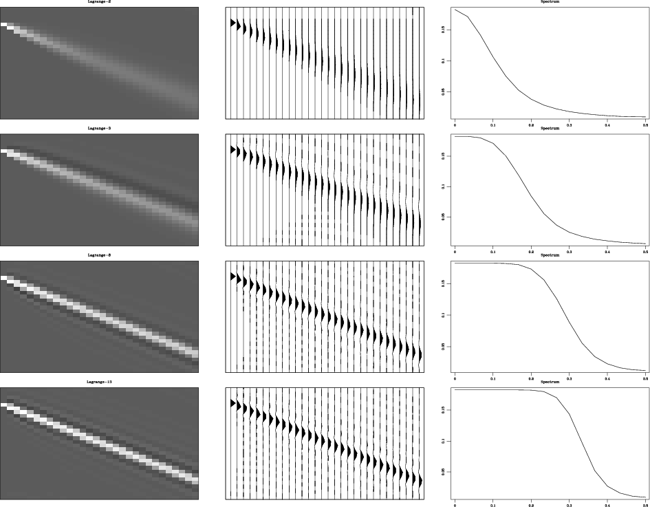
steer-lagrange
Figure 2. Steering filters with Lagrange interpolation. The left and middle plots show the impulse responses of steering filters: the top panel corresponds to linear interpolation (two-point Lagrange, upwind finite-difference); the second top plot, the three-point Lagrange filter (Lax-Wendroff scheme); the two bottom plots, the 8-point and 13-point Lagrange filters. The right plots in each panel show the corresponding average spectrum. The spectrum flattens and the prediction get more accurate with an increase of the filter size.

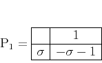
The second-order Taylor approximation yields

$$S_2(Z) = Z^{N_t-1} \left(1 + \sigma (Z-1) {\frac{(\sigma -1) \sigma (Z -1)^2}{2}}\right) =$$

$$\frac{\sigma (\sigma-1)}{2} Z^{T-1} + \left(1-\sigma^2\right) Z^{T} + \frac{\sigma (\sigma+1)}{2} Z^{T+1}\;,$$ (11)

which corresponds to the 2-D filter

$$\mathbf{P}_2 = \begin{array}{\vert c\vert c\vert c\vert}... ...1\right) & -\frac{\sigma (\sigma+1)}{2} \hline \end{array}$$ (12)

and is equivalent to the Lax-Wendroff finite-difference scheme of equation (9). The interpolation, implied by filter (10) is a local three-point polynomial (Lagrange) interpolation. The correspondence of the Taylor series method, described above, and the Lagrange interpolation can be proved by induction. In general, the filter coefficients for the second row of the $N$-th order Lagrangian filter are given by the explicit formula

$$a_{k} = \prod_{i \neq k} \frac{(\sigma-\left[\frac{N}{2}\right]-i)}{(k-i)}\;,$$ (13)

where the $k$ and $i$ range from $0$ to $N$. Such a filter has a stable inverse for $-\frac{N}{2} \le \sigma \le \frac{N+1}{2}$ and additionally produces an exact answer for all integer $\sigma$'s in that range. We would have arrived at the same conclusion if instead of expanding the $Z$-transform of the filter $\mathbf{S}$ around $Z=1$, expanded its Fourier transform around the zero frequency. The latter case corresponds to the ``self-similar'' construction of Karrenbach (1995). The impulse responses for the helix inverses of different-order Lagrangian filters are shown in Figure 2.

If instead of Taylor series in $Z$, we use a rational (Padè) approximation, the filter will get more than one coefficient in the first row, which corresponds to an implicit finite-difference scheme. For example, the $[1/1]$ Padè approximation is

$$S_1^1 (Z) = \frac {1 + \frac{1 + \sigma}{2} (Z-1)} {1 ... ... \frac {1-\sigma + (1+\sigma) Z} {1+\sigma + (1-\sigma) Z}\;$$ (14)

which leads to the filter

$$\mathbf{P}_1^1 = \begin{array}{\vert c\vert c\vert} \hl... ... \hline \frac{\sigma-1}{1+\sigma} & -1 \hline \end{array}$$ (15)

and corresponds to the Crank-Nicolson implicit scheme.

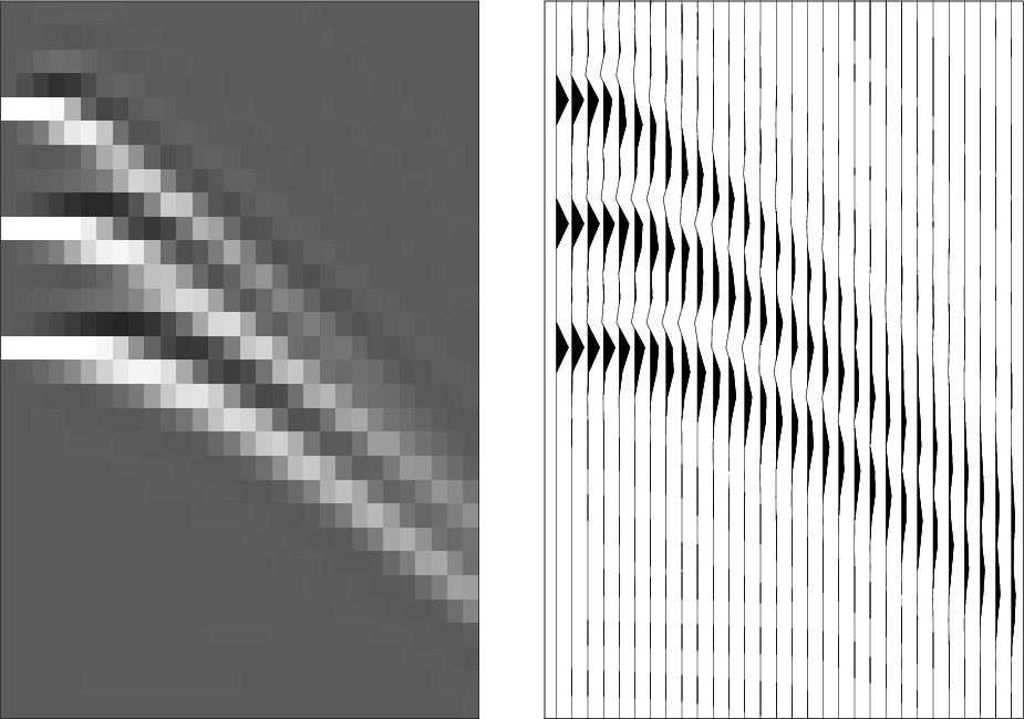
It is interesting to note that a space-variant convolution with inverse plane filters can create signals with different shape, which remains planar only locally. This situation corresponds to a variable slowness $p$ in the one-way wave equation (9). Figure 3 shows an example: predicting hyperbolas with a 7-point Lagrangian filter.

steer-hyp7
Figure 3. Creating hyperbolas with a variant plane-wave prediction: the impulse response of the inverse 7-point time-and-space-variant Lagrangian filter.

Solution steering with space-variant filters