Modeling 3-D anisotropic fractal media

FUTURE WORK

Future goals of this effort will be to formulate the inverse problem for estimating the characteristic parameters of the anisotropic fractal medium, i.e, aspect ratios of anisotropy, and Hausdorff (fractal) dimension. The technique of deriving the binary field from the continuous random field should be extended to simulate M-state models, where M is the number of states or rocks composing an impedance well-log.

I also need to test the method on actual well-log data and demonstrate a better fit with von Karman correlation functions compared to the exponential fit. This would would be the first application of the inverse problem. Two and three dimensional problems can find application in the field of wave scattering and diffraction and in fluid flow problems.

Appendix A

von Karman covariance function

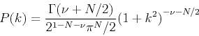
Equation (4) in the text represents the autocovariance of a random medium of fractal nature. The power spectrum of the field corresponds to the Fourier transform of its covariance function:

$$P(k)=\int_{-\infty}^{+\infty}\int_{-\infty}^{+\infty}\int_{-\infty}^{+\infty} C(r)e^{-ik\cdot r} d^3r \$$ (12)

Using the N-dimensional Hankel transform (Lord, 1954), the covariance function and its Fourier transform can be related as follows:

$$p(k)=(2\pi)^{N/2}k^{-N/2+1}\int_{0}^{\infty} r^{N/2}J_{N/2-1}(rk)C(r)dr \$$ (13)

$$C(r)=(2\pi)^{-N/2}r^{-N/2+1}\int_{0}^{\infty} k^{N/2}J_{N/2-1}(rk)P(k)dk \$$ (14)

where $J_{N/2-1}$ is the Bessel function of order $N/2-1$.
The covariance $C(r)$ in (3) is specified in terms of the function:

$$G_\nu (r)=r^\nu K_\nu (r) \hspace{.3in} 0\leq r < \infty \hspace{.3in} \nu \in [0,1]\$$ (15)

whose Hankel transform pair has been derived by Lord (1954):

$$P(k)=\frac {\Gamma{(\nu +N/2)}} {2^{1-N-\nu}\pi{^N/2}} {(1+k^2)}^{-\nu-N/2} \$$ (16)

where $\Gamma$ is the gamma function defined as:

$$\Gamma (z)= \int_{0}^{\infty} t^{z-1}e^{-t} dt \$$ (17)

Finally if we normalize $G_\nu (r)$ by $G_\nu (0)$ as in Goff and Jordan (1988), we obtain, for the three-dimensional case, the power spectrum of the field whose covariance is defined by (4):

$$P(k)=4\pi\nu H^2 {(1+k^2)}^{(-\nu-3/2)} \$$ (18)

Modeling 3-D anisotropic fractal media