Seismic AVO analysis of methane hydrate structures

IMPEDANCE ESTIMATION

The P- and S-impedance contrasts at each subsurface position were estimated by applying a least-squares elastic parameter inversion method (Lumley and Beydoun, 1991; Lumley, 1993) to the CMP gathers. This technique fits the prestack migrated AVO gathers at each pseudo-depth and surface position to the theoretical P- and S-impedance curves which are based on linearized Zoeppritz equations. The least-squares impedance inversion results of the preprocessed CMP gathers are shown in Figures 12 and 13.

pimp-ann
Figure 12. P-impedance contrast section.

simp-ann
Figure 13. S-impedance contrast section.

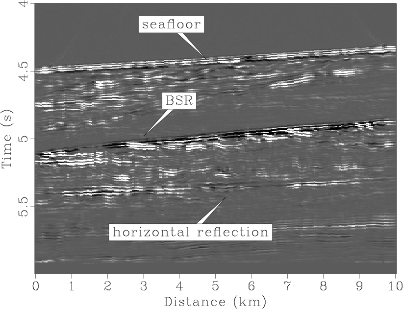
The P-impedance contrast section shows clearly that the seafloor reflection and the BSR have P-impedance contrasts of opposite polarity and approximately the same magnitude. In a small section above the BSR there is a ``quiet'' zone where no diffractions or reflections are visible, which can possibly be explained by the presence of disseminated methane hydrate. The S-impedance section is dominated by a very strong impedance contrast at the BSR. Although the seafloor has a much weaker impedance contrast, it is evident that both have the same polarity. Below the BSR, a horizontal reflector gives a strong P-impedance contrast of the same polarity as the seafloor, indicating an increase in P-wave velocity at the reflector, but weak S-impedance. This may be indicative of the base of the gas zone.

Assuming a seafloor reflection of 0.2 and assuming the P- and S-impedance contrasts at the seafloor, it is possible to estimate the relative impedance contrasts of the BSR by determining the average amplitude changes between seafloor and BSR. This results in a P-impedance contrast of $-$0.4 at the BSR which has the same magnitude but opposite polarity to the seafloor. The S-impedance contrast is very strong and amounts to approximately 0.8 to 1.2, which is two to three times as much as the seafloor impedance contrast of the same polarity. This anomalous S-impedance behavior is even more pronounced by making a simple P$*$S anomaly map shown in Figure 14. Normal impedance structure is plotted dark grey, while anomalous impedance structure is indicated by white. The high magnitude contrast has the effect of visually diminishing the S-impedance contrast of the seafloor (Figure 13) compared with the P-impedance contrast (figure 12) at the seafloor, which are actually the same magnitude.

PSmap-ann
Figure 14. P$*$S impedance contrast.

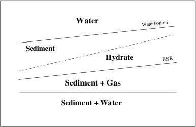
The negative P-impedance contrast and the large positive S-impedance contrast at the BSR are in good agreement with the prediction based on the Zoeppritz modeling. The strong positive S-impedance contrast clearly supports the modeled S-wave velocity behavior of anomalously low S-velocity in the hydrates and considerably increased S-velocity in the underlain gas sediments. Based on the synthetic modeling and the impedance inversion results, the geology was interpreted as seen in Figure 15. In this interpretation, the hydrate-bearing sediments are assumed to overlay sediments in which free gas is trapped. The flat reflector below the BSR might correspond to a gas-water contact at the base of the free gas zone based on the impedance contrasts obtained for this reflector.

interp
Figure 15. Interpretation of the methane hydrate seismic data from the Blake Outer Ridge.

Seismic AVO analysis of methane hydrate structures