Time-lapse image registration using the local similarity attribute

2-D synthetic data

time2-over,mdif-time2-over,dif-time2-over,dif2-time2-over
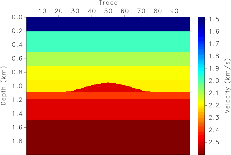
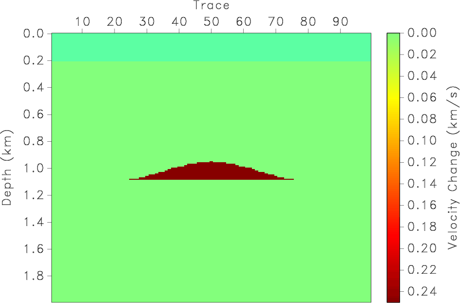
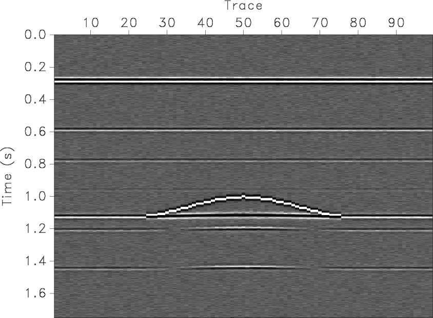
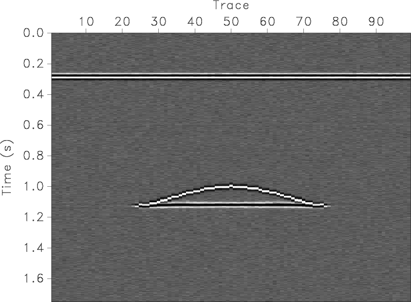
Figure 4. (a) Synthetic model. (b) Time-lapse change containing differences in both the reservoir interval and the shallow overburden. (c) Initial time-lapse difference image. (d) Time-lapse difference image after registration.

scan-time2-over
Figure 5. Local similarity scan for the 2-D synthetic model.

Figure 4(a) shows a more complicated 2-D synthetic example. In this experiment, we assume that the changes occur both in the reservoir and in the shallow subsurface [Figure 4(b)]. The synthetic data were generated by convolution modeling. After computing local similarity between the two synthetic time-lapse images [Figure 5], we apply the extracted stretch factor to register the images. Figures 4(c) and 4(d) compare time-lapse difference images before and after registration. Similarity-based registration effectively removes artifact differences both above and below the synthetic reservoir. As mentioned before, the local similarity cube is an important attribute by itself and includes information on uncertainty bounds for the local stretch factor, which reflects the uncertainty of the reservoir parameter estimation.

Time-lapse image registration using the local similarity attribute