Time-frequency analysis of seismic data using local attributes

2D data example for low-frequency anomaly detection

Low-frequency anomalies are often attributed to abnormally high attenuation in gas-filled reservoirs and can be used as a hydrocarbon indicator (Castagna et al., 2003). A number of studies have investigated possible mechanisms of low-frequency anomalies associated with hydrocarbon reservoirs, but no adequate explanation is accepted absolutely (Ebrom, 2004; Kazemeini et al., 2009).

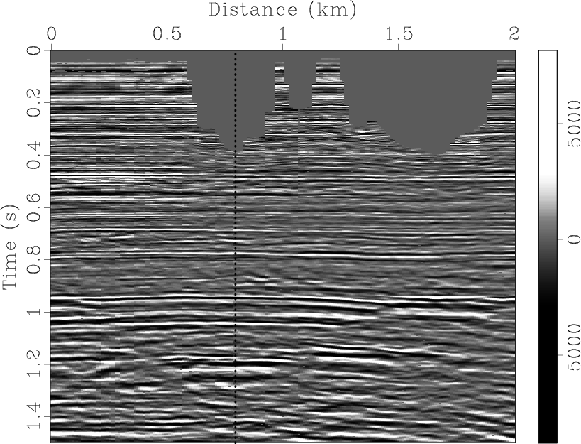
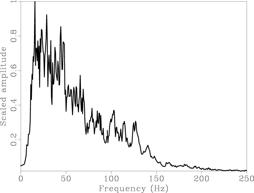
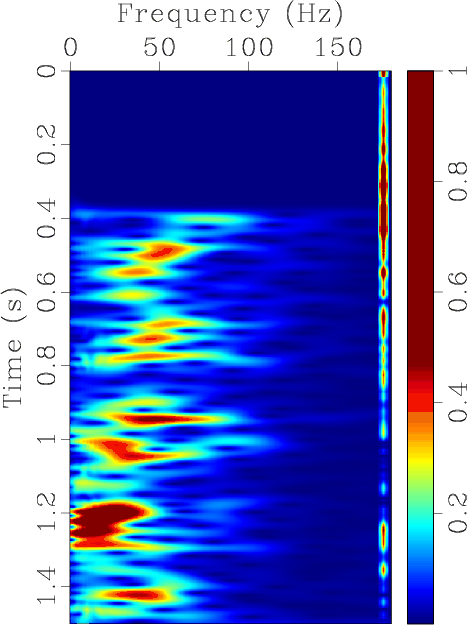
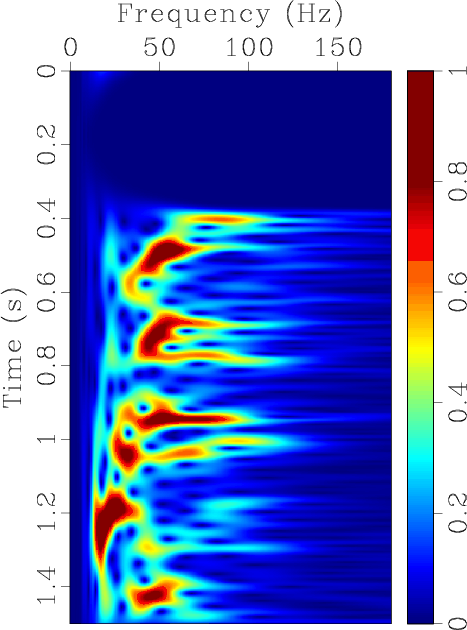
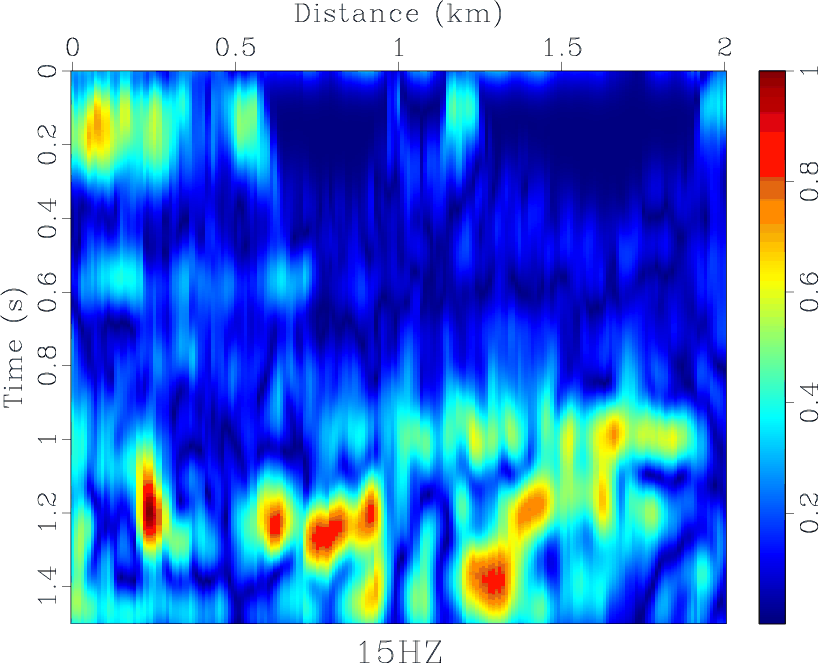
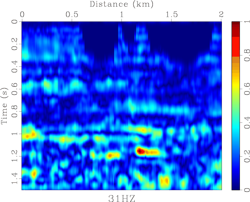
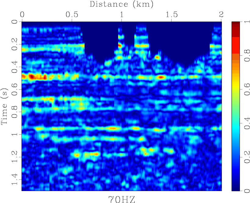
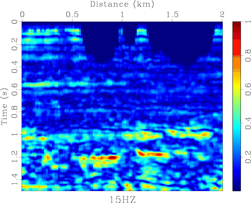
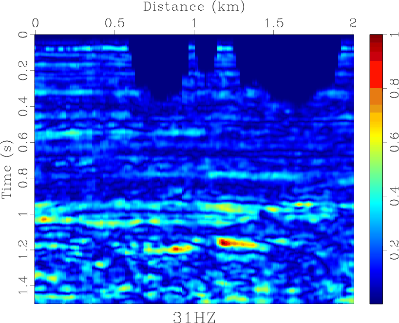
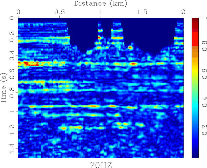
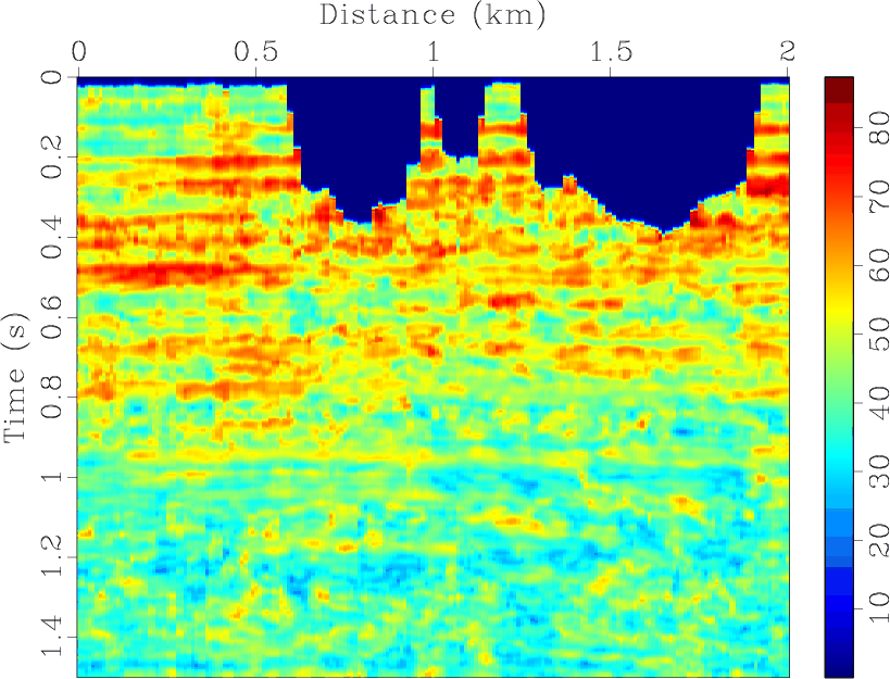
Figure 11 shows a poststack field data set with a bandwidth of about 10–150 Hz (Figure 12).We used our proposed method with a ten-point smoothing radius to generate a time-frequency spectral map. Figure 13 shows the time-frequency map of one trace from the field data set. Note that our method has a higher temporal resolution than that of the S-transform, especially at 0.6-0.8 s.We can observe a general decay of frequency with time caused by seismic attenuation from the time-frequency map of one trace (Figure 13). The low-frequency anomaly is shown at 1.2-1.3 s (arrows). Figures 14 and 15 show single-frequency sections at 15, 31, and 70 Hz from two methods, the S-transform and the proposed method. We further found that the proposed method provides higher temporal and spatial resolution, especially in low-frequency sections. Figures 14(a) and 15(a) both show high-amplitude, low-frequency anomalies (ellipse). However, these anomalies gradually disappear in the high-frequency section (Figures 14(b) and 14(c) and 15(b) and 14(c)). Note that the spatial resolution of low-frequency anomalies in the proposed method (Figure 15(a)) is higher than that in the S-transform (Figure 14(a)). We also computed the time-varying average frequency section for this example using equation 13 (Figure 16). We find that the average frequency is about 60 Hz in shallow layers, but 25 Hz in deep layers. The average frequency of low-frequency anomalies is very low, just about 15 Hz. This example shows that comparison of single low-frequency sections from the proposed method is able to detect low-frequency anomalies that might be caused by hydrocarbons, as demonstrated in other studies (Castagna et al., 2003; Zhenhua et al., 2008; Korneev et al., 2004). What we demonstrate by this example is that the proposed method can be used to detect low-frequency anomalies in seismic sections. Well control is generally needed to interpret this section more accurately.

old-1
Figure 11. A field marine seismic data set.

spectra
Figure 12. The averaged Fourier spectra of the field data.

tf-l,tf-s
Figure 13. Time-frequency map of one trace (denoted by black line in Figure 12). (a) S-transform; (b) the proposed method.

s1,s2,s3
Figure 14. Comparison of common-frequency slices from S-transform; (a) 10 Hz, (b) 31 Hz, and (c) 70 Hz. The lowfrequency abnormality is indicated by an ellipse.

l1,l2,l3
Figure 15. Comparison of common-frequency slices from the proposed method; (a) 10 Hz, (b) 31 Hz, and (c) 70 Hz. The lowfrequency abnormity is indicated by an ellipse.

lcf-l
Figure 16. Estimated time-varying average frequency of the field data from time-frequency map.

Time-frequency analysis of seismic data using local attributes