Time-to-depth conversion and seismic velocity estimation using time-migration velocity

Field data example

elf-fmg2
Figure 3. (a) Seismic image from North Sea obtained by prestack time migration using velocity continuation (Fomel, 2003). (b) Corresponding time-migration velocity.

vels,elfvxz
Figure 4. Field data example of interval velocity estimation. (a) Dix velocity converted to depth. (b) Estimated velocity model and the corresponding image rays. The image-ray spreading causes significant differences between Dix velocity and true velocity.

img0,img,fmg2
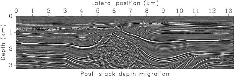
Figure 5. Migrated images of the field data example. (a) Poststack migration using Dix velocity. (b) Poststack migration using estimated velocity. (c) Prestack time migration converted to depth with our algorithm.

Figure 3, taken from (Fomel, 2003), shows a prestack time migrated image from the North Sea and the corresponding time-migration velocity obtained by velocity continuation. The most prominent feature in the image is a salt body which causes significant lateral variations of velocity. Figure 4 compares the Dix velocity converted to depth with the interval velocity model recovered by our method. As in the synthetic example, there is a significant difference between the two velocity caused by the geometrical spreading of image rays. The middle part of the velocity model may not be recovered properly. The true structure should include a salt body visible in the image. The inability of our method to recover it exactly shows the limitation of the proposed approach in the areas of significant lateral velocity variations, which invalidate the assumptions behind time migration (Robein, 2003). Figure 5 compares three images: post-stack depth-migration image using Dix velocity, post-stack depth-migration image using the velocity estimated by our method, and prestack time-migration image converted to depth with our algorithm. The evident structural improvements in Figure 5(b) in comparison with Figure 5(a), in particular near salt flanks, and a good structural agreement between Figures 5(b) and 5(c) serve as an indirect evidence of the algorithm success. An ultimate validation should come from prestack depth migration velocity analysis, which is significantly more expensive.

Time-to-depth conversion and seismic velocity estimation using time-migration velocity