Shaping regularization in geophysical estimation problems

Shaping regularization in theory

The idea of shaping regularization starts with recognizing smoothing as a fundamental operation. In a more general sense, smoothing implies mapping of the input model to the space of admissible functions. I call the mapping operator shaping. Shaping operators do not necessarily smooth the input but they translate it into an acceptable model.

Taking equation 5 and using it as the definition of the regularization operator $\mathbf {D}$, we can write

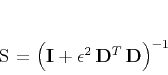$$\mathbf{S} = \left(\mathbf{I} + \epsilon^2\,\mathbf{D}^T\,\mathbf{D}\right)^{-1}$$ (9)

or

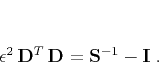$$\epsilon^2\,\mathbf{D}^T\,\mathbf{D} = \mathbf{S}^{-1} - \mathbf{I}\;.$$ (10)

Substituting equation 10 into 1 yields a formal solution of the estimation problem regularized by shaping:

$$\widehat{\mathbf{m}} = \left(\mathbf{L}^T\,\mathbf{L} + \... ...ight)\right]^{-1}\, \mathbf{S}\,\mathbf{L}^T\,\mathbf{d}\;.$$ (11)

The meaning of equation 11 is easy to interpret in some special cases:

• If $\mathbf{S = I}$ (no shaping applied), we obtain the solution of unregularized problem.
• If $\mathbf{L}^T\,\mathbf{L} = \mathbf{I}$ ($\mathbf{L}$ is a unitary operator), the solution is simply $\mathbf{S}\,\mathbf{L}^T\,\mathbf{d}$ and does not require any inversion.
• If $\mathbf{S} = \lambda\,\mathbf{I}$ (shaping by scaling), the solution approaches $\lambda\,\mathbf{L}^T\,\mathbf{d}$ as $\lambda$ goes to zero.

The operator $\mathbf{L}$ may have physical units that require scaling. Introducing scaling of $\mathbf{L}$ by $1/\lambda$ in equation 11, we can rewrite it as

$$\widehat{\mathbf{m}} = \left[\lambda^2\,\mathbf{I} + \m... ...ht) \right]^{-1}\, \mathbf{S}\,\mathbf{L}^T\,\mathbf{d}\;.$$ (12)

The $\lambda$ scaling in equation 12 controls the relative scaling of the forward operator $\mathbf{L}$ but not the shape of the estimated model, which is controlled by the shaping operator $\mathbf{S}$.

Iterative inversion with the conjugate-gradient algorithm requires symmetric positive definite operators (Hestenes and Steifel, 1952). The inverse operator in equation 12 can be symmetrized when the shaping operator is symmetric and representable in the form $\mathbf S = \mathbf{H H}^T$ with a square and invertible $\mathbf {H}$. The symmetric form of equation 12 is

$$\widehat{\mathbf{m}} = \mathbf{H}\,\left[\lambda^2\,\math... ...}\right]^{-1}\, \mathbf{H}^T\,\mathbf{L}^T\,\,\mathbf{d}\;.$$ (13)

When the inverted matrix is positive definite, equation 13 is suitable for an iterative inversion with the conjugate-gradient algorithm. Appendix A contains a complete algorithm description.

Shaping regularization in geophysical estimation problems