|
|
|
|
Lowrank finite-differences and lowrank Fourier finite-differences for seismic wave extrapolation in the acoustic approximation |
Our first example is wave extrapolation in a 2-D, smoothly variable velocity model. The velocity ranges between 500 and 1300 m/s, and is formulated as
| (20) |


|
|---|
|
wavfd7sn,wavel
Figure 4. Wavefield snapshot in a varable velocity field by: (a) conventional 4th-order FD method (b) Lowrank method. |
|
|
It is easy to observe obvious numerical dispersions on the snapshot computed by the 4th-order FD method (Figure 4(a)).
The lowrank FD method with the same order exhibits higher accuracy and fewer dispersion artifacts (Figure 5(a)).
The approximation
rank decomposition in this case is ![]() , with the expected error of
less than
, with the expected error of
less than ![]() .
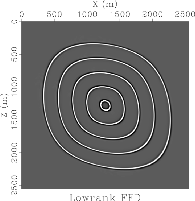
Figure 5(b) displays the snapshot by the 10th-order LFD method with a larger time step:
.
Figure 5(b) displays the snapshot by the 10th-order LFD method with a larger time step:
![]() ms,
ms,
![]() . Note that the result is still accurate. However, the regular FD method becomes unstable in this case.
For comparison, Figure 4(b) displays the snapshot by the lowrank method with the same time step.
The approximation
rank decomposition in this case is
. Note that the result is still accurate. However, the regular FD method becomes unstable in this case.
For comparison, Figure 4(b) displays the snapshot by the lowrank method with the same time step.
The approximation
rank decomposition in this case is ![]() , with the expected error of
less than
, with the expected error of
less than ![]() .
Thanks to the spectral nature of the algorithm, the result appears accurate and free of dispersion artifacts.
.
Thanks to the spectral nature of the algorithm, the result appears accurate and free of dispersion artifacts.


|
|---|
|
wavapp7sn,wavapp10sn
Figure 5. Wavefield snapshot in a varable velocity field by: (a) the 4th-order lowrank FD method (b) the 10th-order lowrank FD method. Note that the time step is 2.5 ms and the LFD result is still accurate. However, the FD method is unstable in this case. |
|
|
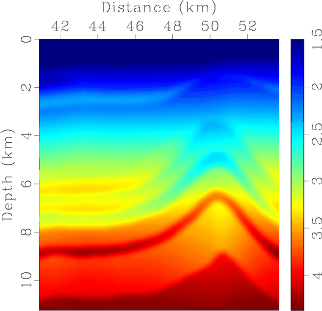
Next, we test the lowrank FD method in a complex velocity model.
Figure 6 shows a part of the BP velocity model (Billette and Brandsberg-Dahl, 2004), which is a complicated model containing a salt body and sharp velocity contrasts on the flanks of the salt body.
We use a Ricker-wavelet at a point source. The dominant frequency is 17 Hz (
![]() ).
The horizontal grid size
).
The horizontal grid size ![]() is 12.5 m, the vertical grid size
is 12.5 m, the vertical grid size ![]() is 12.5 m, and the time step is 1.5 ms.
Thus
is 12.5 m, and the time step is 1.5 ms.
Thus
![]() and
and
![]() .
The approximation
rank decomposition in this case is
.
The approximation
rank decomposition in this case is ![]() , with the expected error of
less than
, with the expected error of
less than ![]() .
In this case, we adopt a disk-shaped compact scheme (8th-order) for LFD with a 4-point radius (
.
In this case, we adopt a disk-shaped compact scheme (8th-order) for LFD with a 4-point radius (
![]() ,
, ![]() ).
Figure 7 displays a wavefield snapshot in the above velocity model.
The snapshot is almost free of dispersions.
This experiment confirms that the lowrank FD method is able to handle sharp velocity variations.
).
Figure 7 displays a wavefield snapshot in the above velocity model.
The snapshot is almost free of dispersions.
This experiment confirms that the lowrank FD method is able to handle sharp velocity variations.

|
|---|
|
sub1
Figure 6. Portion of BP 2004 synthetic velocity model. |
|
|

|
|---|
|
wavsnapabc
Figure 7. Wavefield snapshot by the 8th-order lowrank FD (compact scheme) in the BP Model shown in Figure 6. |
|
|
Our next example is wave propagation in a TTI model with a tilt of ![]() and smooth velocity variation (
and smooth velocity variation (![]() : 800-1225.41 m/s,
: 800-1225.41 m/s, ![]() : 700-883.6 m/s).
Figure 8(a) shows wavefield snapshots at different time steps by a 16th-order LFD operator
in the TTI model.
The space grid size is 5 m and the time step size is 2 ms.
So
: 700-883.6 m/s).
Figure 8(a) shows wavefield snapshots at different time steps by a 16th-order LFD operator
in the TTI model.
The space grid size is 5 m and the time step size is 2 ms.
So
![]() and
and
![]() .
The approximation
rank decomposition in this case is
.
The approximation
rank decomposition in this case is ![]() , with the expected error of
less than
, with the expected error of
less than ![]() .
For TTI model, we adopt a high-order (16th order) LFD operator in order to reduce dispersions.
The scheme is compact and shaped as a disk with a radius of 8 points (
.
For TTI model, we adopt a high-order (16th order) LFD operator in order to reduce dispersions.
The scheme is compact and shaped as a disk with a radius of 8 points (![]() ).
).

|
|---|
|
snapshotlfd,snapshotlffd
Figure 8. Wavefield snapshots in a TTI medium with a tilt of |
|
|
Song and Fomel (2011) showed an application of FFD method for TTI media.
However, the example wavefield snapshot by FFD method still had some dispersion
caused by the fact that the FD scheme in the FFD operator is derived from Taylor's expansion around zero wavenumber.
It was apparent that 4th-order FD scheme is not accurate enough for TTI case
and requires denser sampling per wavelength (
![]() ).
We first apply lowrank approximation
to the mixed-domain velocity correction term in FFD.
The rank is
).
We first apply lowrank approximation
to the mixed-domain velocity correction term in FFD.
The rank is ![]() , with the expected error of
less than
, with the expected error of
less than ![]() .
Then we propose to replace that 4th-order FD operator with an 8th-order LFD compact scheme.
The scheme has the shape of a disk with a radius of 4 points (
.
Then we propose to replace that 4th-order FD operator with an 8th-order LFD compact scheme.
The scheme has the shape of a disk with a radius of 4 points (![]() ), the same as the one for LFD in the above BP model.
Figure 8(b) shows wavefield snapshots by the proposed LFFD operator.
The time step size is 1.5 ms (
), the same as the one for LFD in the above BP model.
Figure 8(b) shows wavefield snapshots by the proposed LFFD operator.
The time step size is 1.5 ms (
![]() ).
Note that the wavefront is clean and almost free of dispersion with
).
Note that the wavefront is clean and almost free of dispersion with
![]() .
Because we use the exact dispersion relation, Equation 17 for TTI computation,
there is no coupling of q-SV wave and q-P wave (Zhang et al., 2009; Grechka et al., 2004; Duveneck et al., 2008) in our snapshots by either LFD or LFFD methods.
.
Because we use the exact dispersion relation, Equation 17 for TTI computation,
there is no coupling of q-SV wave and q-P wave (Zhang et al., 2009; Grechka et al., 2004; Duveneck et al., 2008) in our snapshots by either LFD or LFFD methods.


|
|---|
|
vp0,vx0,yita0,theta0
Figure 9. Partial region of the 2D BP TTI model. a: |
|
|
Next we test the LFD and LFFD methods in a complex TTI model.
Figure 9(a)-9(d) shows parameters for part of the BP 2D TTI model (Shah, 2007).
The dominant frequency is 15 Hz (
![]() ).
The space grid size is 12.5 m and the time step is 1 ms.
Thus
).
The space grid size is 12.5 m and the time step is 1 ms.
Thus
![]() and
and
![]() .
The approximation
rank decomposition for LFD method is
.
The approximation
rank decomposition for LFD method is ![]() , with the expected error of
less than
, with the expected error of
less than ![]() .
For FFD,
.
For FFD, ![]() , with the expected error of
less than
, with the expected error of
less than ![]() .
Both methods are able to simulate an accurate qP-wave field in this model as shown in Figure 10(a) and 10(b).
.
Both methods are able to simulate an accurate qP-wave field in this model as shown in Figure 10(a) and 10(b).


|
|---|
|
snapshotslfd,snapshotslffd
Figure 10. Scalar wavefield snapshots by LFD and LFFD methods in the 2D BP TTI model. |
|
|
It is difficult to provide analytical stability analysis for LFD and LFFD operators.
In our experience, the values of ![]() are around 0.5 for 2D LFD and LFD methods appear to allow for a larger time step size than that of the LFFD method.
In TTI case, the conventional FD method for acoustic TTI has known issues of instability caused by shear-wave numerical artifacts or sharp changes in the symmetry-axis tilting (Zhang et al., 2009; Grechka et al., 2004; Duveneck et al., 2008).
Conventional methods may place limits on anisotropic parameters, smooth parameter models or include a finite shear-wave velocity to alleviate the instability problem(Fletcher et al., 2009; Yoon et al., 2010; Zhang and Zhang, 2008).
Both LFD and LFFD methods are free of shear-wave artifacts.
They require no particular bounds for anisotropic parameters and can also handle sharp tilt changes.
are around 0.5 for 2D LFD and LFD methods appear to allow for a larger time step size than that of the LFFD method.
In TTI case, the conventional FD method for acoustic TTI has known issues of instability caused by shear-wave numerical artifacts or sharp changes in the symmetry-axis tilting (Zhang et al., 2009; Grechka et al., 2004; Duveneck et al., 2008).
Conventional methods may place limits on anisotropic parameters, smooth parameter models or include a finite shear-wave velocity to alleviate the instability problem(Fletcher et al., 2009; Yoon et al., 2010; Zhang and Zhang, 2008).
Both LFD and LFFD methods are free of shear-wave artifacts.
They require no particular bounds for anisotropic parameters and can also handle sharp tilt changes.
|
|
|
|
Lowrank finite-differences and lowrank Fourier finite-differences for seismic wave extrapolation in the acoustic approximation |