 |
 |
 |
 | Lowrank finite-differences and lowrank Fourier finite-differences for seismic wave extrapolation
in the acoustic approximation |  |
![[pdf]](icons/pdf.png) |
Next: Lowrank Finite Differences
Up: Theory
Previous: Theory
The following acoustic-wave equation is widely used in
seismic modeling and reverse-time migration (Etgen et al., 2009):
 |
(1) |
where
 ,
,
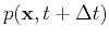
 is the seismic pressure wavefield
and
is the seismic pressure wavefield
and  is the propagation velocity.
Assuming a constant velocity,
is the propagation velocity.
Assuming a constant velocity,  , after Fourier transform in space,
we could obtain the following explicit expression,
, after Fourier transform in space,
we could obtain the following explicit expression,
 |
(2) |
where
 |
(3) |
and
 .
.
Equation 2 has an explicit solution:
 |
(4) |
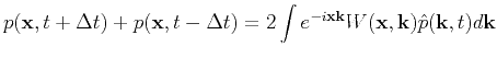
A second-order time-marching scheme and the inverse Fourier transform lead to
the well-known expression (Etgen, 1989; Soubaras and Zhang, 2008) :
 |
(5) |
Equation 5 provides an efficient solution
in the case of a constant-velocity medium with the aid of the fast Fourier transform (FFT).
When velocity varies in space,
equation 5 can provide an approximation by replacing with .
In such a case, a mixed-domain term,
 , appears in the expression.
As a result, the computational cost of a straightforward application of equation 5 is
, appears in the expression.
As a result, the computational cost of a straightforward application of equation 5 is  , where
  is the total size of the three-dimensional space grid.
Fomel et al. (2010,2012) showed that the mixed-domain matrix,
 |
(6) |
can be efficiently decomposed into a separate representation of the following form:
 |
(7) |
where
 is a submatrix of
 that consists of
selected columns associated with
that consists of
selected columns associated with
 ,
,
 is another submatrix that contains
selected rows associated with
is another submatrix that contains
selected rows associated with
 ,
and
,
and  stands for the middle matrix coefficients.
The construction of the separated form 7 follows the method of Engquist and Ying (2009).
The main observation is that the columns of
need to span the column space of the original matrix and that the rows of
need to span the row space as well as possible.
stands for the middle matrix coefficients.
The construction of the separated form 7 follows the method of Engquist and Ying (2009).
The main observation is that the columns of
need to span the column space of the original matrix and that the rows of
need to span the row space as well as possible.
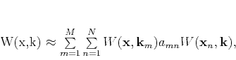
Representation (7) speeds up the computation of
 because
 |
|
|
|
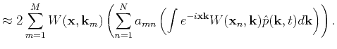 |
|
|
(8) |
Evaluation of equation 8 requires N inverse FFTs.
Correspondingly, the lowrank approximation reduces the cost to
 , where
  is a small integer,
which is related to the rank of the above decomposition
and can be automatically calculated at some given error level with a pre-determined
is a small integer,
which is related to the rank of the above decomposition
and can be automatically calculated at some given error level with a pre-determined  .
Increasing the time step size may increase the rank of the
approximation (
.
Increasing the time step size may increase the rank of the
approximation ( and ) and correspondingly the number of the required Fourier
transforms.
and ) and correspondingly the number of the required Fourier
transforms.
As a spectral method, the lowrank approxmation is highly accurate.
However, its cost is several FFTs per time step.
Our goal is to reduce the cost further by deriving an FD scheme that matches
the spectral response of the output from the lowrank decomposition.
|
|
|
|
| Lowrank finite-differences and lowrank Fourier finite-differences for seismic wave extrapolation
in the acoustic approximation | |
|
Next: Lowrank Finite Differences
Up: Theory
Previous: Theory
2013-06-12