Accelerated plane-wave destruction

Application

The 2D seislet transform (Fomel and Liu, 2010) uses local slopes to predict and update even and odd traces in the wavelet lifting scheme. The seislet transform itself is fast, but the slope estimation step is comparatively slow. The 3D seislet transform can be constructed in the same way by using 3D slopes and cascading 2D transforms in inline and crossline directions. So that an efficient transform can be built, the proposed accelerated plane-wave destruction is applied to slope estimation.

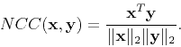
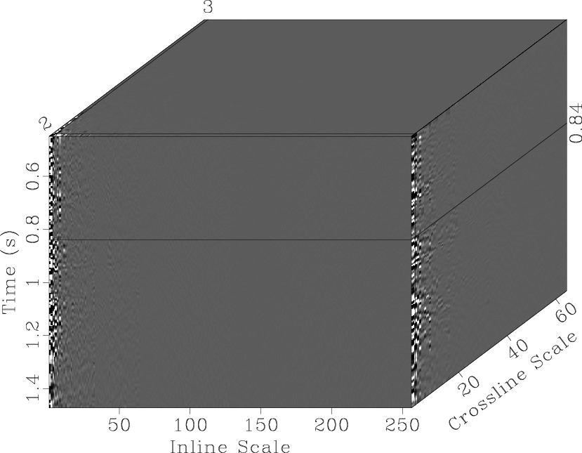
Figure 6 shows a part of the Teapot Dome image from Wyoming. The 3D slope estimation yields two slope fields along two space directions. Figure 7 shows the local inline and crossline slope fields estimated by the proposed algorithm.

The two slopes are used by the lifting scheme in the seislet transform to obtain the seislet transform coefficients. The coefficients of the 2D seislet transform are concentrated at the planes near the zero inline plane, as shown in Figure 8a, whereas in Figure 8b, the 3D transform coefficients are concentrated in the corner region near the origin.

cuber
Figure 6. A portion of the 3D data from the Teapot dataset.

To illustrate the compressive performance of the 3D seislet transform, Figure 9 shows the reconstruction results at different percentages of the compression. Most of the data can be reconstructed using only $1\%$ of the seislet coefficients (1:100 compression ratio). In order to compare with the iterative methods quantitatively, we define the following normalized cross-correlation (NCC)

$$NCC(\mathbf x, \mathbf y) = \frac{\mathbf x^T\mathbf y}{\Vert\mathbf x\Vert _2\Vert\mathbf y\Vert _2}.$$ (23)

fdip1,fdip2
Figure 7. 3D slopes estimated by the proposed algorithm: (a) inline slope, (b) crossline slope.

fseis1,fseis2
Figure 8. Coefficients of: (a) the 2D seislet transform along inline direction only, (b) the 3D seislet transform.

fapprox2,fapprox1
Figure 9. Reconstruction of 3D-seislet-compressed data using: (a) $5\%$ of the seislet coefficients, (b) $1\%$ of the seislet coefficients.

In the seislet transform, the more accurate dip we use, the better compression we can obtain. The NCC between the reconstructed data and the original data can be used to quantify the compressive performance. In Table 1, the proposed method is compared with both three-point ($N=1$) and five-point ($N=2$) iterative methods.

In all the three methods, we use ten-point smoothing windows in both inline and crossline dimensions, and use five-point smoothing window in time direction. In order to obtain a similar slope estimation as the proposed method, the three-point ($N=1$) and five-point ($N=2$) iterative mathods need about six and five iterations respectively. The five-point method can obtain a better compression ratio than the three-point method, because of its better accuracy in slope estimation. However, although the iterative methods have smaller PWD residuals, neighter of them achieves a better NCC than the proposed method. In this case, using the noniterative estimation as the initial in five-point estimation can save at least 250s. That is to say, the computational time cost is reduced by a factor of about 6.

Method	$N$	Iterations	Runtime (s)	RES-inline	RES-xline	NCC-1	NCC-5
noniterative	1	0	54.63	0.2314	0.2242	0.8858	0.9618
iterative	1	6	334.5	0.2267	0.2172	0.8814	0.961
iterative	2	5	301.6	0.2194	0.2075	0.8838	0.9615

Table 1. Performance of different dip estimation methods in 3D seislet transform: Runtime is the run time of the slope estimation process; RES-inline is the inline residual; RES-xline is the crossline residual; NCC-1 is the normalized cross-correlation between the original data and the reconstruction using one percent of the seislet coefficients; NCC-5 uses five percents of the coefficients. The run time for 2D and 3D seislet transform are about 22.45 s and 45.0 s respectively.

Accelerated plane-wave destruction