|
 |
 |
 | Theory of 3-D angle gathers in wave-equation seismic imaging |  |
![[pdf]](icons/pdf.png) |
Next: Common-azimuth approximation
Up: Fomel: 3-D angle gathers
Previous: Introduction
Theoretical analysis of angle gathers in downward continuation methods can be
reduced to analyzing the geometry of reflection in the simple case of a
dipping reflector in a locally homogeneous medium. Considering the reflection
geometry in the case of a plane reflector is sufficient for deriving
relationships for local reflection traveltime derivatives in the vicinity of a
reflection point (Goldin, 2002). Let the local reflection plane be described in
 coordinates by the general equation
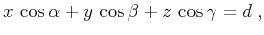 |
(1) |
where the normal angles  ,
,  , and
, and  satisfy
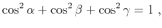 |
(2) |
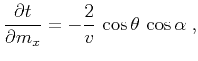
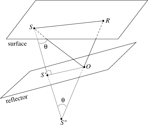
The geometry of the reflection ray paths is depicted in
Figure 1. The reflection traveltime measured on a
horizontal surface above the reflector is given by the known expression
(Slotnick, 1959; Levin, 1971)
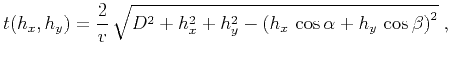 |
(3) |
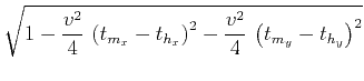
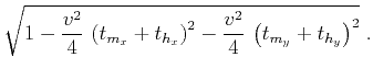
where  is the length of the normal to the reflector from the
midpoint (distance
is the length of the normal to the reflector from the
midpoint (distance  in Figure 2)
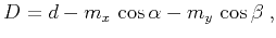 |
(4) |
 and
and  are the midpoint coordinates,
  and
and  are the
half-offset coordinates, and
are the
half-offset coordinates, and  is the local propagation velocity.
|
|---|
plane3b
Figure 1. Reflection geometry in 3-D (a scheme).
 and
and  and the source and the receiver positions at the surface.
  is
the reflection point.
is
the reflection point.  is the normal projection of the source to the
reflector.
is the normal projection of the source to the
reflector.  is the ``mirror'' source. The cumulative length of the
incident and reflected rays is equal to the distance from
to
.
is the ``mirror'' source. The cumulative length of the
incident and reflected rays is equal to the distance from
to
.
|
|---|
![[png]](icons/viewmag.png) ![[xfig]](icons/xfig.png)
|
|---|
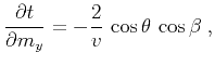
According to elementary geometrical considerations
(Figures 1 and 2), the reflection angle  is related to the previously introduced quantities by the equation
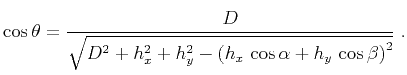 |
(5) |

|
|---|
plane2b
Figure 2. Reflection geometry in the reflection
plane (a scheme).  is the midpoint. As follows from the similarity of
triangles
is the midpoint. As follows from the similarity of
triangles  and
and  , the distance from
to
is twice smaller
than the distance from
to
.
, the distance from
to
is twice smaller
than the distance from
to
.
|
|---|
|
|
|---|
Explicitly differentiating equation (3) with respect to the
midpoint and offset coordinates and utilizing equation (5)
leads to the equations
Additionally, the traveltime derivative with respect to the depth of the
observation surface is given by
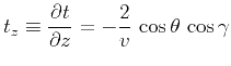 |
(10) |
and is related to the previously defined derivatives by the double-square-root
equation
In the frequency-wavenumber domain, equation (11) serves as the
basis for 3-D shot-geophone downward-continuation imaging. In the Fourier
domain, each  derivative translates into
 ratio, where
  is the wavenumber corresponding to
  and
and  is the temporal frequency.
Equations (6), (7), and (10) immediately
produce the first important 3-D relationship for angle gathers
 |
(12) |
Expressing the depth derivative with the help of the double-square-root
equation (11) and applying a number of algebraic transformations,
one can turn equation (12) into the dispersion relationship
 |
(13) |
For each reflection angle
and each frequency
,
equation (13) specifies the locations on the
four-dimensional ( ,
,  ,
,  ,
,  )
wavenumber hyperplane that contribute to the common-angle gather. In
the 2-D case, equation (13) simplifies by setting
and
)
wavenumber hyperplane that contribute to the common-angle gather. In
the 2-D case, equation (13) simplifies by setting
and  to zero. Using the notation
 and
and
 , the 2-D equation takes the form
 |
(14) |
and can be explicitly solved for  resulting in the convenient
2-D dispersion relationship
resulting in the convenient
2-D dispersion relationship
 |
(15) |
In the next section, I show that a similar simplification is also valid
under the common-azimuth approximation. Equations (13)
and (15) describe an effective migration of the
downward-continued data to the appropriate positions on midpoint-offset planes
to remove the structural dependence from the local image gathers.
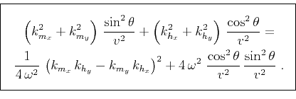
Another important relationship follows from eliminating the local velocity
from equations (11) and (12). Expressing  from
equation (12) and substituting the result in
equation (11), we arrive (after a number of algebraical
transformations) to the frequency-independent equation
from
equation (12) and substituting the result in
equation (11), we arrive (after a number of algebraical
transformations) to the frequency-independent equation
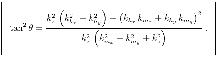 |
(16) |
Equation (16) can be expressed in terms of ratios
 and
and
 , which correspond at the zero local offset to local
structural dips (
, which correspond at the zero local offset to local
structural dips ( and
and  partial derivatives), and ratios
 and
and
 , which correspond to local offset slopes. As shown by Sava and Fomel (2005), it can be also expressed as
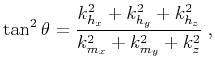 |
(17) |
where  refers to the vertical offset between source and receiver wavefields (Biondi and Shan, 2002).
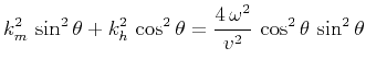
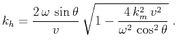
In the 2-D case, equation (16) simplifies to the form,
independent of the structural dip:
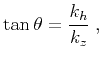 |
(18) |
which is the equation suggested by Sava and Fomel (2003).
Equation (18) appeared previously in the theory of
migration-inversion (Stolt and Weglein, 1985).
|
|
|
|
| Theory of 3-D angle gathers in wave-equation seismic imaging | |
|
Next: Common-azimuth approximation
Up: Fomel: 3-D angle gathers
Previous: Introduction
2013-03-02