Streaming orthogonal prediction filter in $t$ -$x$ domain for random noise attenuation

Shot gather

The second synthetic model was created by Guochang Liu (Liu et al., 2012). The shot gather (Figure 5a) has four hyperbolic events and 501 traces. Figure 5b is the noisy data containing random noise. The denoised result from the $f$ -$x$ deconvolution (Figure 6a) still contains lots of random noise. There is also signal leakage in the removed noise (Figure 6b). For $f$ -$x$ RNA, we set the filter length as 10 samples and the smoothing radius as 3 samples (in frequency) $\times$ 20 samples (in space). Figure 7b shows that $f$ -$x$ RNA has a good denoising performance in the shot gather test. However, it creates some artificial events with weak energy, which are parallel with the events (Figure 7a). As for the $t$ -$x$ space-noncausal SOPF, the filter size is 11 samples (in time) $\times$ 6 samples (in space) and the scale parameters are 2.0 ($\lambda_t$ ), 0.8 ($\lambda_x$ ), 0.4 ($\gamma_t$ ), and 1.0 ($\gamma_x$ ), respectively. The comparison of Figure 7a and 8a illustrates that the SOPF has similar signal preservation ability to $f$ -$x$ RNA. Careful examination indicates that the shaping regularization (Fomel, 2007) in the $f$ -$x$ RNA has a more powerful smoothing effect than the streaming method. Figures 7b and 8b show that the SOPF also eliminates equivalent random noise compared with the $f$ -$x$ RNA. However, the proposed method is still removing some signal along with the noise; we can preserve more signal by selecting smaller values for $\lambda$ in equation 9. Users can therefore decide whether to choose more noise attenuation or more signal preservation to meet their data processing objectives. The computational cost of the SOPF is much less than that of $f$ -$x$ RNA because no iteration is used in the proposed method. For further illustrating how filtering methods change the amplitudes of the original signal, we calculate the differences between the clean data (Figure 5a) and the denoised results by the nonstationary $f$ -$x$ RNA (Figure 7a) or $t$ -$x$ SOPF (Figure 8a). The results are shown in Figure 9. The comparison shows the proposed method provides more reasonable signal preservation than the nonstationary $f$ -$x$ RNA.

gpara,gnpara
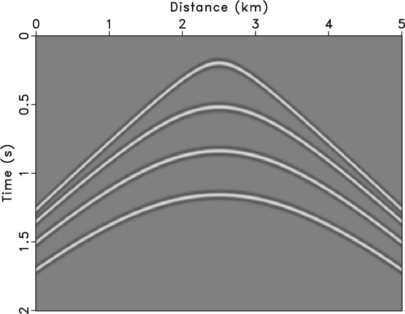
Figure 5. Shot gather (a) and noisy data (b).

gfx,gfxn2
Figure 6. Denoised result by the $f$ -$x$ deconvolution (a) and noise removed by the $f$ -$x$ deconvolution (b).

grna,grnan2
Figure 7. Denoised result by the $f$ -$x$ RNA (a) and noise removed by the $f$ -$x$ RNA (b).

gh2,gr2
Figure 8. Denoised result by the $t$ -$x$ SOPF (a) and noise removed by the $t$ -$x$ SOPF (b).

diff1,diff2
Figure 9. Comparison of the difference between Figure 5a and the corresponding denoised result using two different methods, the nonstationary $f$ -$x$ RNA (Figure 7a) (a) and the $t$ -$x$ SOPF (Figure 8a) (b).

Streaming orthogonal prediction filter in $t$ -$x$ domain for random noise attenuation