|
|
|
|
Basic operators and adjoints |
There is a huge gap between the conception of an idea and putting it into practice. During development, things fail far more often than not. Often, when something fails, many tests are needed to track down the cause of failure. Maybe the cause cannot even be found. More insidiously, failure may be below the threshold of detection and poor performance suffered for years. The dot-product test enables us to ascertain if the program for the adjoint of an operator is precisely consistent with the operator. It can be, and it should be.
Conceptually, the idea of matrix transposition is simply
![]() .
In practice, however, we often encounter matrices far too large
to fit in the memory of any computer.
Sometimes it is also not obvious how to formulate the process at hand
as a matrix multiplication.
(Examples are differential equations and fast Fourier transforms.)
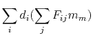
What we find in practice is that an operator and its adjoint
are two routines.
The first amounts to the matrix multiplication
.
In practice, however, we often encounter matrices far too large
to fit in the memory of any computer.
Sometimes it is also not obvious how to formulate the process at hand
as a matrix multiplication.
(Examples are differential equations and fast Fourier transforms.)
What we find in practice is that an operator and its adjoint
are two routines.
The first amounts to the matrix multiplication
![]() .
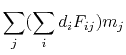
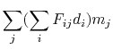
The adjoint routine computes
.
The adjoint routine computes
![]() ,
where
,
where ![]() is the conjugate-transpose matrix.
In later chapters we solve huge sets of simultaneous equations
in which both routines are required.
If the pair of routines are inconsistent,
we may be doomed from the start.
The dot-product test is a simple test for verifying that the two
routines are adjoint to each other.
is the conjugate-transpose matrix.
In later chapters we solve huge sets of simultaneous equations
in which both routines are required.
If the pair of routines are inconsistent,
we may be doomed from the start.
The dot-product test is a simple test for verifying that the two
routines are adjoint to each other.
I will tell you first what the dot-product test is,
and then explain how it works.
Take a model space vector ![]() filled with random numbers, and likewise
a data space vector
filled with random numbers, and likewise
a data space vector ![]() filled with random numbers.
Use your forward modeling code to compute:
filled with random numbers.
Use your forward modeling code to compute:
| (31) | |||
| (32) | |||
| (33) | |||
| (34) |
| (35) |
 |
 |
(38) | |
 |
(39) | ||
| (40) | |||
| (41) |
The program for applying the dot product test is dottest
![]() .
The C way of passing a linear operator
as an argument is to specify the function interface. Fortunately, we
have already defined the interface for a generic linear operator. To
use the dottest program, you need to initialize an operator
with specific arguments (the _init subroutine) and then pass
the operator itself (the _lop function) to the test program.
You also need to specify the sizes of the model and data vectors so
that temporary arrays can be constructed. The program runs the dot
product test twice, the second time with add = true to test if
the operator can be used properly for accumulating results, for example.
.
The C way of passing a linear operator
as an argument is to specify the function interface. Fortunately, we
have already defined the interface for a generic linear operator. To
use the dottest program, you need to initialize an operator
with specific arguments (the _init subroutine) and then pass
the operator itself (the _lop function) to the test program.
You also need to specify the sizes of the model and data vectors so
that temporary arrays can be constructed. The program runs the dot
product test twice, the second time with add = true to test if
the operator can be used properly for accumulating results, for example.
![]() .
.
    /* < L m1, d2 > = < m1, L* d2 > (w/o add) */
    oper(false, false, nm, nd, mod1, dat1);
    dot1[0] = cblas_dsdot( nd, dat1, 1, dat2, 1);

    oper(true, false, nm, nd, mod2, dat2);
    dot1[1] = cblas_dsdot( nm, mod1, 1, mod2, 1);

    /* < L m1, d2 > = < m1, L* d2 > (w/  add) */
    oper(false, true, nm, nd, mod1, dat1);
    dot2[0] = cblas_dsdot( nd, dat1, 1, dat2, 1);

    oper(true, true, nm, nd, mod2, dat2);
    dot2[1] = cblas_dsdot( nm, mod1, 1, mod2, 1);
|
I ran the dot product test on many operators
and was surprised and delighted to find
that for small operators
it is generally satisfied to an accuracy near the computing precision.
For large operators, precision can become and issue.
Every time I encountered a relative discrepancy of ![]() or more
on a small operator (small data and model spaces),
I was later able to uncover a conceptual or programming error.
Naturally,
when I run dot-product tests, I scale the implied matrix to a
small size both
to speed things along and to be sure that
boundaries are not overwhelmed by the much larger interior.
or more
on a small operator (small data and model spaces),
I was later able to uncover a conceptual or programming error.
Naturally,
when I run dot-product tests, I scale the implied matrix to a
small size both
to speed things along and to be sure that
boundaries are not overwhelmed by the much larger interior.
Do not be alarmed if the operator you have defined has truncation errors. Such errors in the definition of the original operator should be matched by like errors in the adjoint operator. If your code passes the dot-product test, then you really have coded the adjoint operator. In that case, to obtain inverse operators, you can take advantage of the standard methods of mathematics.
We can speak of a continuous function ![]() or a discrete function
or a discrete function ![]() .
For continuous functions, we use integration;
and for discrete ones, we use summation.
In formal mathematics, the dot-product test
defines the adjoint operator,
except that the summation in the dot product
may need to be changed to an integral.
The input or the output or both can be given
either on a continuum or in a discrete domain.
Therefore, the dot-product test
.
For continuous functions, we use integration;
and for discrete ones, we use summation.
In formal mathematics, the dot-product test
defines the adjoint operator,
except that the summation in the dot product
may need to be changed to an integral.
The input or the output or both can be given
either on a continuum or in a discrete domain.
Therefore, the dot-product test
![]() could have an integration on one side of the equal sign
and a summation on the other.
Linear-operator theory is rich with concepts not developed here.
could have an integration on one side of the equal sign
and a summation on the other.
Linear-operator theory is rich with concepts not developed here.
|
|
|
|
Basic operators and adjoints |