Pluto Model

Velocity Models

The Pluto model was designed to offer a complex environment to test multiple attenuation algorithms. The model is 32 km (105,000 ft) long and 9.14 km (30,000 ft) in deep.

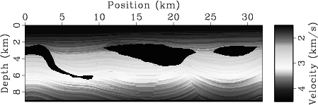
The velocity model file int_depth_vp.sgy has 1201 datapoints in the vertical direction and 6960 datums in the horizontal direction. The actual synthetic surveys were conducted on a padded model which contains constant velocity cells outside of the model boundaries.

To assure the proper geometry Pluto velocity model headers should be formatted as shown in table 2. Values are listed for both metric and standard units. This article will display metric units exclusively.

Standard
n1=1201	n2=6960	d1=0.025	d2=0.025	o1=0	o2=-34.875
Metric
n1=1201	n2=6960	d1=.0076	d2=.0076	o1=0	o2=-10.629
Padded
n1=1401	n2=6960	d1=.025 or .0076	d2=.025 or .0076	o1=0	o2=-34.875 or -10.629

Table 2. Header information for Pluto velocity models

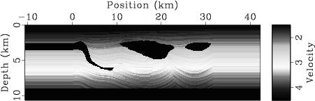
TheSConstruct file found within rsf/book/data/pluto is shown in table 3. This SConstruct file produces both metric and standard plots of the velocity model. However, only the metric one is presented here in figure 1. Additionally, the padded model found in file P15VPint_25f_padded.SEGY, is displayed in figure 2 for reference.

from rsf.proj import *
# Fetch Files from repository
Fetch("int_depth_vp.sgy","pluto")
Fetch("P15VPint_25f_padded.SEGY","pluto")

# Convert Files to RSF
Flow('velocityProfileStd','int_depth_vp.sgy',
     '''
     segyread read=d |
     put  d2=.025 label1=Depth o2=-34.875 
     label2=Position unit1=kft unit2=kft 
     label=Velocity unit=kft/s |
     scale rscale=0.001
     ''')

Flow('velocityProfileMetric','int_depth_vp.sgy',
     '''
     segyread read=d |
     put d1=.00760 d2=.00760 o2=-10.629
     label1=Depth label2=Position label=Velocity 
     unit1=km unit2=km unit=km/s |
     scale rscale=.0003048
     ''')

Flow('velocityProfilePadded','P15VPint_25f_padded.SEGY',
     '''
     segyread read=d |
     put  d1=.0076 d2=.00760 o2=-10.629 label1=Depth
     label2=Position unit1=km unit2=km label=Velocity |
     scale rscale=.0003048
     ''')

# Plotting Section
mins=[0,0,-10.5]
maxs=['105','32','42.5']

counter=0
for item in ['Std','Metric']:
    Result('velocityProfile' + item,
           '''
           window j1=2 j2=2 |
           grey scalebar=y color=j allpos=y bias=1 title=P-Wave Velocity Profile
           max2=%s min2=0 screenratio=.28125 screenht=2 
           labelsz=4 wanttitle=n barreverse=y
           ''' % maxs[counter])
    counter=counter+1

Result('velocityProfilePadded',
       '''
       window j1=2 j2=2 |
       grey scalebar=y color=j allpos=y bias=1 gainpanel=a title=P-Wave Velocity Profile
       screenratio=.28 125 screenht=2 labelsz=4 wanttitle=n barreverse=y 
       ''')

End()

Table 3. SConstruct script generating the velocity model images

Typing command 1 within the pluto directory runs the script.

$$\texttt{bash-3.1\$\ scons\ view}$$ (1)

velocityProfileMetric
Figure 1. Pluto P-wave velocity model in metric units

velocityProfilePadded
Figure 2. Padded velocity model that surveys were conducted on

Pluto Model