Imaging overturning reflections by Riemannian Wavefield Extrapolation

Riemannian wavefield extrapolation

Riemannian wavefield extrapolation (Sava and Fomel, 2005) generalizes solutions to the Helmholtz equation of the acoustic wave-equation

$$\Delta \mathcal{U}=-\omega ^2 s^2 \mathcal{U}\;,$$ (1)

to non-Cartesian coordinate systems, such that extrapolation is not performed strictly in the downward direction. In equation (1), $s$ is slowness, $\omega$ is temporal frequency, and $\mathcal{U}$ is a monochromatic acoustic wave.

Assume that we describe the physical space in Cartesian coordinates $x$, $y$ and $z$, and that we describe a Riemannian coordinate system using coordinates $\xi$, $\eta$ and $\zeta$ related through a generic mapping

$$x = x \left (\xi ,\eta ,\zeta \right )\;,$$ (2)

$$y = y \left (\xi ,\eta ,\zeta \right )\;,$$ (3)

$$z = z \left (\xi ,\eta ,\zeta \right )\;,$$ (4)

which allows us to compute derivatives of the Cartesian coordinates relative to the Riemannian coordinates.

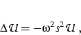
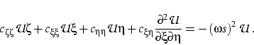
Following the derivation of Sava and Fomel (2005), the acoustic wave-equation in Riemannian coordinates can be written as:

$$c_{\zeta \zeta }\dtwo{\mathcal{U}}{\zeta } + c_{\xi \xi }\dt... ...\partial \eta } = - \left (\omega s \right )^2 \mathcal{U}\;.$$ (5)

where coefficients $c_{ij}$ are spatially-variable functions of the coordinate system and can be computed numerically for any given coordinate system using the mappings (2)-(4).

The acoustic wave-equation in Riemannian coordinates (5) ignores the influence of first order terms present in a more general acoustic wave-equation in Riemannian coordinates. This approximation is justified by the fact that, according to the theory of characteristics for second-order hyperbolic equations (Courant and Hilbert, 1989), the first-order terms affect only the amplitude of the propagating waves.

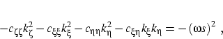
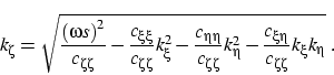
From equation (5) we can derive a dispersion relation of the acoustic wave-equation in Riemannian coordinates

$$- c_{\zeta \zeta }k_\zeta ^2 - c_{\xi \xi }k_\xi ^2 - c_{\et... ... c_{\xi \eta }k_\xi k_\eta = - \left (\omega s \right )^2 \;,$$ (6)

where $k_\zeta$, $k_\xi$ and $k_\eta$ are wavenumbers associated with the Riemannian coordinates $\zeta$, $\xi$ and $\eta$. For one-way wavefield extrapolation, we need to solve the quadratic equation (6) for the wavenumber of the extrapolation direction $k_\zeta$, and select the solution with the appropriate sign for the desired extrapolation direction:

$$k_\zeta = \sqrt{ \frac{ \left (\omega s\right )^2}{c_{\zeta... ...^2 - \frac{c_{\xi \eta }}{c_{\zeta \zeta }}k_\xi k_\eta }\;.$$ (7)

The coordinate system coefficients $c_{ij}$ and the extrapolation slowness $s$ can be combined to form a reduced set of parameters. In 2D, for example, all coordinate-system coefficients can be represented by 2 parameters, $a$ and $b$. Further extensions and implementation details of equation (7) are described by Sava and Fomel (2006).

Extrapolation using equation (7) implies that the coefficients defining the medium and coordinate system are not changing spatially. In this case, we ca perform extrapolation using a simple phase-shift operation

$$\mathcal{U}_{{ \tau}+\Delta{ \tau}} = \mathcal{U}_{{ \tau}} e^{i k_\tau \Delta{ \tau}} \;,$$ (8)

where $\mathcal{U}_{\tau +\Delta\tau }$ and $\mathcal{U}_{\tau }$ represent the acoustic wavefield at two successive extrapolation steps, and $k_\tau$ is the extrapolation wavenumber defined by equation (7).

For media with variability of the coefficients $c_{ij}$ due to either velocity variation or focusing/defocusing of the coordinate system, we cannot use in extrapolation the wavenumber computed directly using equation (7). Like for the case of extrapolation in Cartesian coordinates, we can approximate the wavenumber $k_\tau$ using series expansions relative to coefficients $c_{ij}$ present in the dispersion relation (7). Such approximations can be implemented in the space-domain, in the Fourier domain or in mixed space-Fourier domains (Sava and Fomel, 2006).

Imaging overturning reflections by Riemannian Wavefield Extrapolation