Elastic wave-mode separation for TTI media

Wave-mode separation for symmetry planes of VTI media

Dellinger and Etgen (1990) separate quasi-P and quasi-SV modes in 2D VTI media by projecting the wavefields onto the directions in which P and S modes are polarized. For example, in the wavenumber domain, one can project the wavefields onto the P-wave polarization vectors $W_P$ to obtain quasi-P (qP) waves:

$$\widetilde{{\it q}P}=i W_P({\bf k}) \cdot \widetilde{\mathbf W} =i U_x \widetilde W_x+i U_z \widetilde W_z ,$$ (1)

where $\widetilde{{\it q}P}$ is the P-wave mode in the wavenumber domain, ${\bf k}=\{k_x,k_z\}$ is the wavenumber vector, $\widetilde{\mathbf W}$ is the elastic wavefield in the wavenumber domain, and $W_P({\bf k})$ is the P-wave polarization vector as a function of the wavenumber ${\bf k}$ .

The polarization vectors $W({\bf k})$ of plane waves for VTI media in the symmetry planes can be found by solving the Christoffel equation  (Aki and Richards, 2002; Tsvankin, 2005):

$$\left [{\bf G} - \rho V^2 {\bf I} \right]W= 0 ,$$ (2)

where G is the Christoffel matrix with $G_{ij}=c_{ijkl}n_jn_l$ , in which $c_{ijkl}$ is the stiffness tensor. The vector $\mathbf n=\frac{{\bf k}}{\left\vert{\bf k}\right\vert}$ is the unit vector orthogonal to the plane wavefront, with $n_j$ and $n_l$ being the components in the $j$ and $l$ directions, $i,j,k,l=1,2,3$ . The eigenvalues $V$ of this system correspond to the phase velocities of different wave-modes and are dependent on the plane wave propagation direction $\mathbf k$ .

For plane waves in the vertical symmetry plane of a TTI medium, since qP and qSV modes are decoupled from the SH-mode and polarized in the symmetry planes, one can set $n_y=0$ and obtain

$$\left [ \mtrx{ G_{11}-\rho V^2 & G_{12}\ G_{12} & G_{22} -\rho V^2 } \right] \left [\mtrx{ U_x\ U_z} \right] =0 ,$$ (3)

where

$$G_{11} = c_{11} n_x^2 +c_{55} n_z^2 ,$$ (4)

$$G_{12} = \left (c_{13}+c_{55}\right)n_xn_z ,$$ (5)

$$G_{22} = c_{55} n_x^2 +c_{33} n_z^2 .$$ (6)

Equation 3 allows one to compute the polarization vectors $W_P=\{U_x,U_z\}$ and $W_{SV}=\{-U_z,U_x\}$ (the eigenvectors of the matrix G) given the stiffness tensor at every location of the medium.

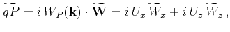
Equation 1 represents the separation process for the P-mode in 2D homogeneous VTI media. To separate wave-modes for heterogeneous models, one needs to use different polarization vectors at every location of the model (Yan and Sava, 2009), because the polarization vectors change spatially with medium parameters. In the space domain, an expression equivalent to equation 1 at each grid point is

$${\it q}P=\nabla_a\cdot \mathbf W= L_x[W_x] + L_z[W_z] ,$$ (7)

where $L\left [ \cdot \right]$ indicates spatial filtering, and $L_x$ and $L_z$ are the filters to separate P waves representing the inverse Fourier transforms of $i U_x$ and $i U_z$ , respectively. The terms $L_x$ and $L_z$ define the ``pseudo-derivative operators'' in the $x$ and $z$ directions for a VTI medium, respectively, and they change according to the material parameters, $V_{P0}$ , $V_{S0}$ ($V_{P0}$ and $V_{S0}$ are the P and S velocities along the symmetry axis, respectively), $\epsilon$ , and $\delta$  (Thomsen, 1986).

Elastic wave-mode separation for TTI media