Interferometric imaging condition for wave-equation migration

Noise model

Consider a medium whose behavior is completely defined by the acoustic velocity, i.e. assume that the density 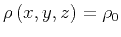$\rho \left (x,y,z \right)= \rho_0$ is constant and the velocity $v \left (x,y,z \right)$ fluctuates around a homogenized value $v_0 \left (x,y,z\right)$ according to the relation

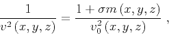$$\frac{1} {v^2 \left (x,y,z \right)} = \frac{1 + \sigma m \left (x,y,z \right)}{v_0^2 \left (x,y,z \right)}\;,$$ (12)

where the parameter $m$ characterizes the type of random fluctuations present in the velocity model, and $\sigma$ denotes their strength.

Consider the covariance orientation vectors

$${\bf a} = \left (a_x,a_y,a_z\right)^{\top} \in \mathbb{R}^3$$ (13)

$${\bf b} = \left (b_x,b_y,b_z\right)^{\top} \in \mathbb{R}^3$$ (14)

$${\bf c} = \left (c_x,c_y,c_z\right)^{\top} \in \mathbb{R}^3$$ (15)

defining a coordinate system of arbitrary orientation in space. Let $r_a, r_b, r_c > 0$ be the covariance range parameters in the directions of ${\bf a}$,${\bf b}$ and ${\bf c}$, respectively.

We define a covariance function

$$\mathrm{cov} \left (x,y,z \right)= \exp \left [-l^{\alpha} \left (x,y,z \right)\right]\;,$$ (16)

where $\alpha \in [0,2]$ is a distribution shape parameter and

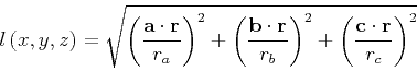$$l \left (x,y,z \right)= \sqrt{\left (\frac{{\bf a}\cdot {\b... ...ight)^2 + \left (\frac{{\bf c}\cdot {\bf r}}{r_c} \right)^2}$$ (17)

is the distance from a point at coordinates ${\bf r}=\left (x,y,z \right)$ to the origin in the coordinate system defined by $\{r_a {\bf a}, r_b {\bf b}, r_c {\bf c}\}$.

Given the IID Gaussian noise field $n \left (x,y,z \right)$, we obtain the random noise $m \left (x,y,z \right)$ according to the relation

$$m \left (x,y,z \right)= \mathscr{F}^{-1} \left [\sqrt{\wideh... ...ight)} \; \widehat{ n} \left (k_x,k_y,k_z \right) \right]\;,$$ (18)

where $k_x,k_y,k_z$ are wavenumbers associated with the spatial coordinates $x,y,z$, respectively. Here,

$$\widehat{\mathrm{cov}} = \mathscr{F} \left [\mathrm{cov}\right]$$ (19)

$$\widehat{n} = \mathscr{F} \left [n \right]$$ (20)

are Fourier transforms of the covariance function $\mathrm{cov}$ and the noise $n$, $\mathscr{F}[\cdot]$ denotes Fourier transform, and $\mathscr{F}^{-1}[\cdot]$ denotes inverse Fourier transform. The parameter $\alpha$ controls the visual pattern of the field, and ${\bf a},{\bf b},{\bf c}, r_a,r_b,r_c$ control the size and orientation of a typical random inhomogeneity.

Interferometric imaging condition for wave-equation migration