|
|
|
|
Waves in strata |
We could work out the mathematical problem
of finding an analytic solution for
the travel time
as a function of distance in an earth with stratified ![]() ,
but the more difficult problem is
the practical one which is the reverse,
finding
,
but the more difficult problem is
the practical one which is the reverse,
finding ![]() from the travel time curves.
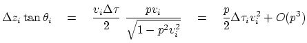
Mathematically we can
express the travel time (squared)
as a power series in distance
from the travel time curves.
Mathematically we can
express the travel time (squared)
as a power series in distance ![]() .
Since everything is symmetric in
.
Since everything is symmetric in ![]() ,
we have only even powers.
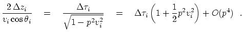
The practitioner's approach is to look at small offsets
and thus ignore
,
we have only even powers.
The practitioner's approach is to look at small offsets
and thus ignore ![]() and higher powers.
Velocity then enters only as the coefficient of
and higher powers.
Velocity then enters only as the coefficient of ![]() .
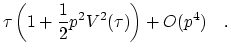
Let us why it is the RMS velocity,
equation (3.25),
that enters this coefficient.
.
Let us why it is the RMS velocity,
equation (3.25),
that enters this coefficient.
The hyperbolic form of equation (3.24) will generally not be exact
when ![]() is very large.
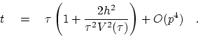
For ``sufficiently'' small
is very large.
For ``sufficiently'' small ![]() ,
the derivation of the hyperbolic shape follows
from application of Snell's law at each interface.
Snell's law implies that the Snell parameter
,
the derivation of the hyperbolic shape follows
from application of Snell's law at each interface.
Snell's law implies that the Snell parameter ![]() , defined by
, defined by
 |
(41) |
XXXXXXXX
|
|
|
|
Waves in strata |